In my previous post in the 5G NR RAN series, I showed how to decode the PDCCH (physical downlink control channel), which is used to send control information from the gNB (base station) to the UEs (cellphones). In this series I am using as an example a short recording of the downlink of an srsRAN gNB. The PDCCH transmission that I decoded in the previous post was a DCI (downlink control information) containing the scheduling of the SIB1 PDSCH transmission. The PDSCH is the physical downlink shared channel, which is the channel where the gNB transmits data. The SIB1 is the system information block 1. It contains basic information about the cell, and it is decoded by the UE after decoding the MIB in the PBCH, as part of the cell attach procedure. In this post I will show how to decode this PDSCH SIB1 transmission.
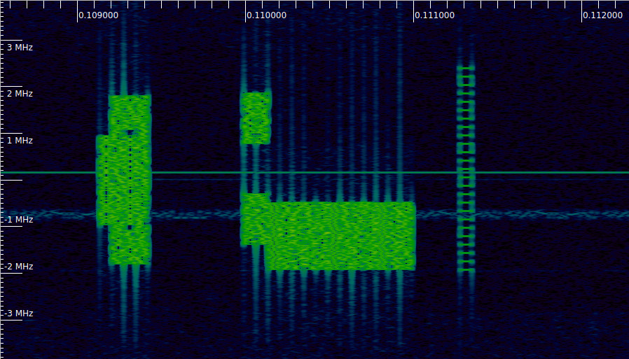
The PDSCH transmission that we will use in this post is shown in the following Inspectrum waterfall. It begins approximately at 0.1102 seconds and occupies the lower part of the 5 MHz cell. The transmission immediately before it (starting at 0.11 seconds), which is split into two blocks in frequency, is the corresponding scheduling in the PDCCH, which I decoded in the previous post. This is the only PDSCH transmission in the IQ recording I am using. Since there are no UEs attached to the cell, the gNB is only transmitting broadcast data and signals.
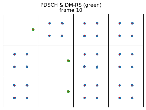
In the post about the downlink reference signals I showed how to generate the PDSCH DM-RS (demodulation reference signal) pseudorandom sequence, and produced the following constellation plot. The plot contains one time-domain symbol per square. The duration of this PDSCH transmission is 12 symbols, which are symbols 2 through 13 in the subframe. Symbols 2, 7 and 11 are used by the DM-RS, which is shown in green with the pseudorandom sequence wiped off. The remaining 9 symbols contain QPSK data.
PDSCH encoding
Before proceeding to decode this PDSCH transmission, let us review how the PDSCH is encoded. The input to the PDSCH channel coding is a transport block. The transport block contains the data to be transmitted, and perhaps some padding, since the transport block size needs to be chosen from a list of possible choices. The receiver finds the transport block size indirectly by using the MCS transmitted in the PDCCH scheduling (which determines the target coding rate and the constellation) and the number of resource elements assigned to PDSCH data. We will look at this process in more detail below.
The PDSCH channel coding is described in Section 7.2 in TS 38.212. First, a CRC is attached to the end of the transport block. For transport blocks longer than 3824 bits, the CRC is a CRC-24, while for transport blocks shorter or equal than 3824 bits, the CRC is a CRC-16.
The PDSCH uses LDPC as FEC. There are two base graphs that are used to build the parity check matrix using a protograph construction. These are called base graph 1 and base graph 2. The rules for how to choose the base graph are given in Section 7.2.2 in TS 38.212. Base graph 2 is used in each of the three following cases:
- \(A \leq 292\)
- \(A \leq 3824\) and \(R \leq 0.67\)
- \(R \leq 0.25\)
Here \(A\) denotes the transport block size in bits and \(R\) denotes the target coding rate given by the MCS. Base graph 1 is used in any other case.
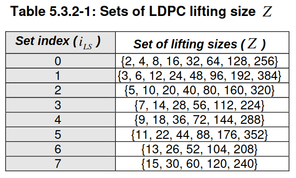
Each of the two base graphs can be lifted by each of the lifting sizes \(Z_c\) given in the table below to generate a Tanner graph that has \(Z_c\) times the number of vertices as the protograph.
The resulting LDPC code is an \((N, K)\) code with \(N = 66Z_c\) and \(K = 22Z_c\) (code rate 1/3) for base graph 1, and \(N = 50Z_c\) and \(K = 10Z_c\) (code rate 1/5) for base graph 2. All these LDPC codes use puncturing, so the number of variable nodes in the graph is actually \(N + 2Z_c\). The first \(2Z_c\) codeword bits are punctured.
Before LDPC encoding, the transport block with its attached CRC needs to be segmented into code blocks. This procedure is described in Section 5.2.2 of TS 38.212. Essentially, it involves splitting the transport block into one or multiple code blocks, each of which is smaller than the maximum code block size, which is \(K_{\mathrm{cb}} = 8448\) for base graph 1 and \(K_{\mathrm{cb}} = 3840\) for base graph 2. If multiple code blocks are needed, a CRC-24 is attached to each of them.
As part of the code block segmentation process, the appropriate lifting size \(Z_c\) is determined. The general rule is that if \(K’\) is the number of bits per code block, then \(Z_c\) is chosen as the smallest lifting size that satisfies \(K_bZ_c \geq K’\), where \(K_b = 22\) for base graph 1 and \(K_b = 10\) for base graph 2. This is quite straightforward, because it is the same as choosing the smallest possible \(K\) that is greater or equal to \(K’\). However, for base graph 2 and short transport blocks, an alternative definition of \(K_b\) is used. If \(B\) denotes the number of bits in the transport block plus CRC, then \(K_b\) is set to 9 for \(560 < B \leq 640\), to 8 for \(192 < B \leq 560\), and to 6 for \(B \leq 192\). Note that this amounts to choosing a \(Z_c\) which is strictly larger than needed. For instance, for \(B = 192\), without this rule we would choose \(Z_c = 20\), which gives \(K = 200\), which is already larger than \(B\). However, this rule says that we need to satisfy \(6 Z_c \geq 192\), so we need to choose \(Z_c = 32\), which gives \(K = 320\).
The code blocks are padded with <NULL> symbols to obtain \(K\) bits. These <NULL> symbols are treated as zeros in the LDPC encoder, but they are never transmitted over the air. Since the locations of <NULL> symbols are known to the receiver beforehand (from the knowledge of the transport block size), it can treat them as known bits during LDPC decoding. In this way, the rule given above for choosing \(K_b < 10\) with base graph 2 and \(B \leq 640\) is forcing a lower code rate for short transport blocks by adding known bits (This code rate reduction affects only the LDPC code. Rate matching still operates to obtain a coding rate that is close to the target rate.)
Each \(K\)-bit code block is encoded by the \((N, K)\) LDPC code determined by the choice of base graph and lifting size \(Z_c\). The LDPC codes are systematic, so the first \(K\) variable nodes correspond to the \(K\)-bit information code block. The first \(2 Z_c\) bits of the systematic part are always punctured. As mentioned above, <NULL> symbols are treated as zeros for the purpose of the calculation of the parity check symbols, but they are preserved as <NULL>s in the systematic output so that they can be removed in the rate matching step.
The construction of the LDPC code from the base graph is a quasi-cyclic protograph construction. This means that each one in the parity check matrix of the base graph is replaced by a circular shift of a \(Z_c \times Z_c\) identity matrix, and each zero in the parity check matrix of the base graph is replaced by a \(Z_c \times Z_c\) zero matrix. Two tables in TS 38.212 Section 5.3.2 define the positions of the ones in the parity check matrices of the two base graphs, and indicate which circular shift needs to be applied to each identity matrix when lifting the code by a factor of \(Z_c\). The circular shifts depend on the index \(i_{\mathrm{LS}}\) associated with \(Z_c\) in the table shown above.
After each code block has been LDPC encoded to give an \(N\)-bit coded block, each of these is rate matched separately to obtain \(E_r\) bits, where \(r\) denotes the code block index. In the simplest case of only one code block, \(E_0 = E\) is given by the number of bits available in the PDSCH transmission, which depends on the number of resource elements used for data symbols and on the constellation (modulation order). If there are multiple code blocks, an algorithm in Section 5.4.2.1 explains how the bits are distributed to each code block.
Rate matching is performed in two steps: bit selection and bit interleaving. In the bit selection step, the coded block is written into a circular buffer of size \(N_{\mathrm{cb}}\). Generally, \(N_{\mathrm{cb}} = N\), so the coded block is fully written into the buffer. However, in some cases there is the possibility of using a reduced \(N_{\mathrm{cb}} < N\) (limited-buffer rate matching), in which case only the beginning of the coded block is written into the buffer and the remaining part is directly punctured. The bit selection algorithm involves going through the circular buffer starting at index \(k_0\) and copying non-<NULL> bits to the output and jumping over <NULL> bits until \(E\) output bits have been produced.
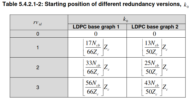
The starting index \(k_0\) is chosen in terms of the redundancy version \(rv_{\mathrm{id}}\). Recall that in a HARQ system each time that the receiver requests a retransmission because it failed to decode the data, new FEC information is sent, enabling the receiver to improve its decoding (instead of transmitting the same data again). In LTE and 5G this is achieved by using the redundancy version (which is a 2-bit integer) to select which part of the FEC encoder output is transmitted. The formulas for \(k_0\) are shown in the following table.
The bit interleaving step works as a matrix interleaver. Bits are written by rows on a matrix with \(Q_m\) rows and \(E/Q_m\) columns, where \(Q_m\) is the modulation order (the number of bits per constellation symbol), and then read by columns. After rate matching is performed for each code block, all the outputs are concatenated, giving a \(G\)-bit sequence.
The physical layer of the PDSCH is described in Section 7.3.1 in TS 38.211. A PDSCH transmission can transmit up to two codewords, \(q = 0, 1\), simultaneously by using MIMO. The simplest case is when only one codeword is transmitted. The codewords are first scrambled with a pseudorandom sequence generated using the initialization value \(n_{\mathrm{RNTI}}\cdot2^{15} + q\cdot2^{14} + n_{\mathrm{ID}}\), where \(n_{\mathrm{RNTI}}\) is the RNTI, and \(n_{\mathrm{ID}}\) is the physical cell ID, \(N_{\mathrm{ID}}^{\mathrm{cell}}\), unless overridden by upper layer configuration. Then the codewords are modulated with a modulation that is chosen according to the MCS. It can be QPSK, 16QAM, 64QAM, 256QAM or 1024QAM.
The modulated codewords are mapped to layers and then to antenna ports. In this recording this is very simple, because the gNB only has one antenna port, so there is only one layer, and the mapping is straightforward. Finally, the symbols are mapped to the resource elements that are allocated to the PDSCH data symbols. In this mapping there can be additional complications regarding mapping from virtual resource blocks to physical resource blocks, but we can ignore these for this recording.
Transport block size and related calculations
To start decoding a PDSCH transmission, the first thing we need to do is to figure out the transport block size. Essentially, this is determined by the MCS, which gives the target coding rate \(R\) and the modulation order \(Q_m\), and by the number of resource elements allocated to PDSCH data.
The exact calculations for the number of resource elements allocated to PDSCH data, \(N_{\mathrm{RE}}\) are in Section 5.1.3.2 in TS 38.214. They are somewhat more complex that simply counting resource elements in the time-frequency grid, because they involve an overhead \(N_{\mathrm{oh}}^{\mathrm{PRB}}\) and a minimum number of resource elements per resource block. However, in many cases including this one, the calculations give the same value as counting resource elements on the time-frequency grid directly. In this case, the math is simple. There are 9 symbols used by PDSCH data and the transmission occupies 8 resource blocks, so the total number of data resource elements is \(N_{\mathrm{RE}} = 9 \cdot 8 \cdot 12 = 864\).
In the previous post we decoded the DCI corresponding to this PDSCH transmission and saw that it uses MCS 5. Looking this value up in the appropriate table gave us \(Q_m = 2\) (QPSK modulation) and \(R = 379/1024 \approx 0.37\). We can now continue the calculations in Section 5.1.3.2 in TS 38.214 to obtain that the unquantized number of information bits is \(N_{\mathrm{info}} = N_{\mathrm{RE}}R Q_m \nu\). Here \(\nu\) is the number of layers, which is \(\nu = 1\). Therefore \(N_{\mathrm{info}} = 639.5625\). This is less or equal than 3824, so continuing the calculations for this case we have \(n = \max(3, \lfloor \log_2(N_{\mathrm{info}})\rfloor – 6) = 3\) and \(N_{\mathrm{info}}’ = \max(24, 2^n \cdot \lfloor N_{\mathrm{info}}/2^n\rfloor) = 632\). The transport block size needs to be chosen as the smallest value from Table 5.1.3.2-1 that is greater or equal than \(N_{\mathrm{info}}’\). This gives a transport block size of 640 bits. There is an online transport block size calculator that can be used to verify this result.
Knowing the transport block size \(A = 640\), we can figure out all the details about the LDPC code that is used to encode the transport block. For this transport block size, the CRC size is 16 bits, so \(B = A + 16 = 656\) is the size of the transport block with CRC attached. The base graph choice is base graph 2, since \(A \leq 3824\) and \(R \leq 0.67\). No code block segmentation is needed.
To determine the lifting size \(Z_c\), we note that \(B > 640\), so \(K_b = 10\), and we see that the smallest lifting size that satisfies \(K_b Z_c \geq K’ = B\) is \(Z_c = 72\). This implies that the LDPC code size is \((N, K) = (50Z_c, 10Z_c) = (3600, 720)\).
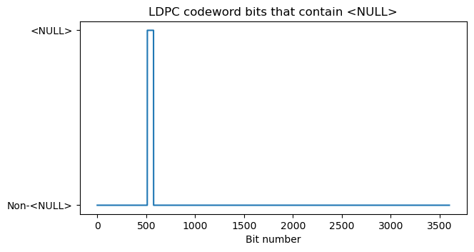
The transport block with CRC is padded with <NULL> symbols to obtain a 720 bit block for the LDPC encoder. This block is systematically encoded, but the first \(2Z_c = 144\) bits are punctured. With this in mind, we know the locations of the <NULL> symbols in the output of the LDPC encoder. These are shown graphically in the following plot.
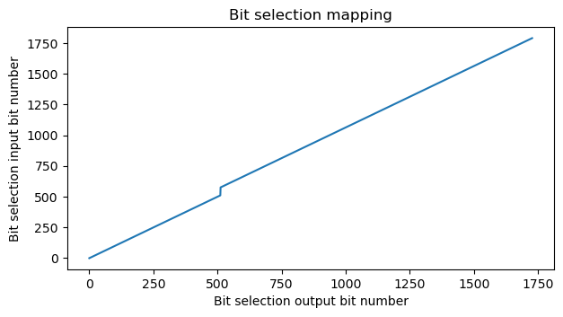
The DCI for this PDSCH transmission indicates that it uses redundancy version 0, which makes sense for a broadcast transmission of the SIB1 in which retransmissions aren’t done and the coding rate is set low enough that any UE that has enough SNR to attach to the cell can decode it. We can perform the bit selection algorithm taking into account the positions of <NULL> symbols in order to see how this selection maps output bits to input bits. Note that the bit selection algorithm needs to select \(E = N_{RE}Q_m = 1728\) bits. The mapping is shown in the next plot. We see that the bit selection starts at bit zero, skips over the <NULL> symbols, and selects a total of 1728 bits from the beginning of the codeword.
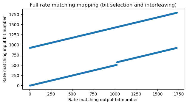
After bit selection, the rate matching algorithm applies bit interleaving. Here we are using \(Q_m = 2\) (QPSK), so the bit interleaving is equivalent to mapping the first half of the data to the real part of the QPSK symbols and the second half to the imaginary part. The output-to-input mapping performed by all the rate matching, including bit interleaving is shown in this plot.
LDPC decoding
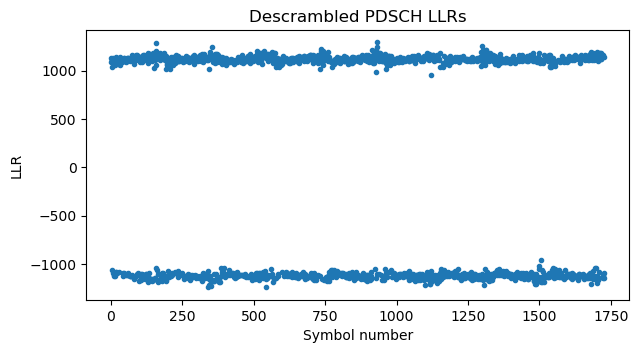
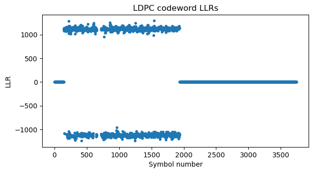
With all these calculations now done, we can begin decoding. First we compute the LLRs of the QPSK symbols and apply descrambling. The initialization value of the scrambling sequence uses the RNTI 0xffff, which is the SI-RNTI, \(q = 0\), since only one codeword is transmitted, and \(n_{\mathrm{ID}} = 1\), which is the physical cell ID. The descrambled LLRs are shown here.
Applying the output-to-input mapping of the rate matching algorithm, we obtain the LLRs for the LDPC codeword. Symbols that have not been transmitted have an LLR of zero. These are the first \(2 Z_c\) symbols, which are always punctured, and all the last symbols, which were discarded by the rate matching algorithm. Note that the LDPC code has rate 1/5 = 0.2, but the target coding rate is 0.37, which is higher, so it is normal that rate matching discards almost half of the codeword bits. There are some LLRs around symbol number 700 that do not appear in this plot. Their LLR is \(+\infty\) because they correspond to <NULL> symbols, so the LDPC decoder can be sure that their value is zero. Note that in this case no LDPC codeword symbol is transmitted multiple times by the rate matching algorithm (which can perform repetition coding when required), so no soft-combining of LLRs is done.
To perform LDPC decoding we need to obtain the parity check matrix of the code for base graph 2 and \(Z_c = 72\). I have implemented generation of the alists for the 5G LPDC codes in my ldpc-toolbox library. The alist file for the code we need can be generated with
ldpc-toolbox 5g --base-graph 2 --lifting-size 72
The Jupyter notebook parses the alist to obtain the parity check matrix.
I could have done LDPC decoding with ldpc-toolbox, but I have decided to write a simple implementation of the sum-product algorithm in the Jupyter notebook. This matches what I have done in other cases for the LTE and 5G series of posts (I already have a Viterbi decoder, a Turbo decoder and a Polar decoder implemented in a few lines of Python in each of the notebooks), and it also allows me to easily plot the LLRs in each decoder iteration to show its progress.
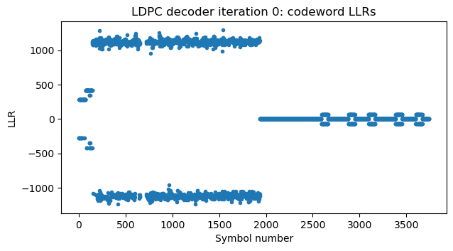
In the first iteration, the LDPC decoder is able to determine all the punctured information bits. Most of the parity check bits that were not transmitted by rate matching remain unsolved.
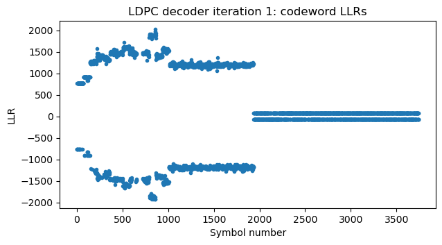
In the second iteration, all the parity check bits are solved, the codeword is valid and the decoder terminates.
SIB1 decoding
After LDPC decoding is done we obtain the transport block with CRC by performing hard decision on the first \(B\) bits of the codeword. We can check the CRC-16 and find that it is correct (this could have also been used as a stopping check for the LDPC decoder, which would have the advantage that it terminates successfully even if there are some errors affecting parity bits only). After checking the CRC-16, we remove it from the transport block.
The transport block contains an ASN.1 BCCH-DL-SCH-Message encoded in UPER. There are some padding bits at the end, since the ASN.1 message needs to be padded to one of the allowed transport block sizes, but these padding bits do not disturb the ASN.1 decoder. The output of the decoder is the following.
{'message': ('c1',
  ('systemInformationBlockType1',
   {'cellSelectionInfo': {'q-RxLevMin': -70, 'q-QualMin': -20},
    'cellAccessRelatedInfo': {'plmn-IdentityInfoList': [{'plmn-IdentityList': [{'mcc': [0,
          0,
          1],
         'mnc': [0, 1]}],
       'trackingAreaCode': (b'\x00\x00\x07', 24),
       'cellIdentity': (b'\x00\x00\x01\x9b\x00', 36),
       'cellReservedForOperatorUse': 'notReserved'}]},
    'connEstFailureControl': {'connEstFailCount': 'n1',
     'connEstFailOffsetValidity': 's30',
     'connEstFailOffset': 1},
    'servingCellConfigCommon': {'downlinkConfigCommon': {'frequencyInfoDL': {'frequencyBandList': [{'freqBandIndicatorNR': 3}],
       'offsetToPointA': 1,
       'scs-SpecificCarrierList': [{'offsetToCarrier': 0,
         'subcarrierSpacing': 'kHz15',
         'carrierBandwidth': 25}]},
      'initialDownlinkBWP': {'genericParameters': {'locationAndBandwidth': 6600,
        'subcarrierSpacing': 'kHz15'},
       'pdcch-ConfigCommon': ('setup',
        {'commonSearchSpaceList': [{'searchSpaceId': 1,
           'controlResourceSetId': 0,
           'monitoringSlotPeriodicityAndOffset': ('sl1', None),
           'monitoringSymbolsWithinSlot': (b'\x80\x00', 14),
           'nrofCandidates': {'aggregationLevel1': 'n0',
            'aggregationLevel2': 'n0',
            'aggregationLevel4': 'n1',
            'aggregationLevel8': 'n0',
            'aggregationLevel16': 'n0'},
           'searchSpaceType': ('common', {'dci-Format0-0-AndFormat1-0': {}})}],
         'searchSpaceSIB1': 0,
         'pagingSearchSpace': 1,
         'ra-SearchSpace': 1}),
       'pdsch-ConfigCommon': ('setup',
        {'pdsch-TimeDomainAllocationList': [{'mappingType': 'typeA',
           'startSymbolAndLength': 53}]})},
      'bcch-Config': {'modificationPeriodCoeff': 'n4'},
      'pcch-Config': {'defaultPagingCycle': 'rf128',
       'nAndPagingFrameOffset': ('oneT', None),
       'ns': 'one'}},
     'uplinkConfigCommon': {'frequencyInfoUL': {'frequencyBandList': [{'freqBandIndicatorNR': 3}],
       'absoluteFrequencyPointA': 355970,
       'scs-SpecificCarrierList': [{'offsetToCarrier': 0,
         'subcarrierSpacing': 'kHz15',
         'carrierBandwidth': 25}]},
      'initialUplinkBWP': {'genericParameters': {'locationAndBandwidth': 6600,
        'subcarrierSpacing': 'kHz15'},
       'rach-ConfigCommon': ('setup',
        {'rach-ConfigGeneric': {'prach-ConfigurationIndex': 1,
          'msg1-FDM': 'one',
          'msg1-FrequencyStart': 4,
          'zeroCorrelationZoneConfig': 0,
          'preambleReceivedTargetPower': -100,
          'preambleTransMax': 'n7',
          'powerRampingStep': 'dB4',
          'ra-ResponseWindow': 'sl10'},
         'ssb-perRACH-OccasionAndCB-PreamblesPerSSB': ('one', 'n4'),
         'ra-ContentionResolutionTimer': 'sf64',
         'prach-RootSequenceIndex': ('l839', 1),
         'restrictedSetConfig': 'unrestrictedSet'}),
       'pusch-ConfigCommon': ('setup',
        {'pusch-TimeDomainAllocationList': [{'k2': 4,
           'mappingType': 'typeA',
           'startSymbolAndLength': 27}],
         'msg3-DeltaPreamble': 6,
         'p0-NominalWithGrant': -76}),
       'pucch-ConfigCommon': ('setup',
        {'pucch-ResourceCommon': 11,
         'pucch-GroupHopping': 'neither',
         'p0-nominal': -90})},
      'timeAlignmentTimerCommon': 'infinity'},
     'n-TimingAdvanceOffset': 'n25600',
     'ssb-PositionsInBurst': {'inOneGroup': (b'\x80', 8)},
     'ssb-PeriodicityServingCell': 'ms10',
     'ss-PBCH-BlockPower': -16},
    'ue-TimersAndConstants': {'t300': 'ms1000',
     't301': 'ms1000',
     't310': 'ms1000',
     'n310': 'n1',
     't311': 'ms30000',
     'n311': 'n1',
     't319': 'ms1000'}}))}
There is a lot to unpack here, so let me comment on some of the most interesting fields. All the definitions of RRC messages are in TS 38.331.
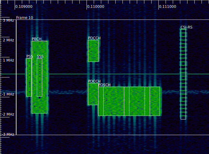
The downlinkConfigCommon says that freqBandIndicatorNR is 3. This means that the cell uses the band n3, which has 1805 – 1880 MHz as downlink. This is correct. For instance, the lowest subcarrier of the SSB has a nominal frequency of 1875.150 MHz in this recording. The offsetToPointA is 1. This is the distance, in resource blocks, between PointA and the lowest resource block of the SSB. PointA is used as the frequency reference for many elements in 5G and corresponds to the centre of the lowest subcarrier of common resource block 0.
We can see this in effect in the following waterfall. We had seen in the previous post that \(k_{\mathrm{SSB}} = 8\). This gives the distance in subcarriers between the lowest subcarrier of the SSB and the lowest subcarrier of CORESET0, which is where the SIB1 is transmitted. We can see that the lower edge of the PDSCH SIB1 transmission is 8 subcarriers lower than the lower edge of the SSB. The cell actually begins one resource block lower, as evidenced by the bounding box of the CSI-RS (this CSI-RS only uses the highest subcarrier in each resource block, which is why the bounding box appears to begin too low).
The scs-SpecificCarrierList defines a carrier that starts at PointA (offsetToCarrier is zero) and uses 15 kHz subcarrier spacing and 25 resource blocks. This matches what we know about the bandwidth of the cell, and in fact this carrier is fully occupied by the CSI-RS and CSI-RS TRS.
The initialDownlinkBWP defines the same carrier. Its locationAndBandwidth, which is 6600 is a RIV (resource indicator value) that needs to be parsed as we did for the DCI format 1_0 in the previous post, using \(N_{\mathrm{BWP}}^{\mathrm{size}} = 275\). This gives \(L_{\mathrm{RBs}} = 25\) and \(RB_{\mathrm{start}} = 0\), which again corresponds to 25 resource blocks starting at PointA.
The uplinkConfigCommon also describes a 25-resource block cell in the n3 band. It contains an absoluteFrequencyPointA equal to 355970. Using this online ARFCN calculator we see that 355970 corresponds to 1779.85 MHz, which is in the uplink of the n3 TDD band. The corresponding downlink frequency is ARFCN 374970, which is 1874.85 MHz. Above I mentioned that the lowest subcarrier of the SSB is at 1875.150 MHz. The downlink PointA is 8 subcarriers and one resource block below this, so it is at 1874.85 MHz, as expected from the uplink ARFCN.
In the pdsch-TimeDomainAllocationList, the startSymbolAndLength contains a SLIV (start and length indicator value), which is a number that contains both the starting symbol and the length in symbols of the PDSCH. As defined in Section 5.1.2.1 of TS 38.214, the SLIV is encoded in a similar way to the RIV. Denoting by \(S\) and \(L\) the start and length respectively, if \(L – 1 \leq 7\), then \(SLIV = 14 \cdot (L – 1) + S\). Otherwise, \(SLIV = 14 \cdot (14 – L + 1) + (14 – 1 – S)\). In this case, the SLIV is 53, which corresponds to \(S = 2\), \(L = 12\), which is something we already knew about the PDSCH configuration.
The PUSCH (physical uplink shared channel) has startSymbolAndLength equal to 27. This SLIV corresponds to \(S = 0\), \(L = 14\). This makes sense because the uplink doesn’t have to reserve a few symbols at the beginning of the slot for the control channel, so the PUSCH can occupy the 14 symbols of the slot.
The ssb-PositionsInBurst field contains configuration about the SSB transmissions. The inOneGroup field is a bitmap that indicates which SS/PBCH blocks are actually transmitted. In this case, the bitmap is 0x80, and only the first 4 bits are valid because the cell has 15 kHz sub-carrier spacing and the carrier frequency is below 3 GHz, so there is a maximum 4 SSB candidates. The bitmap 0x80 means that only the first SSB in each group is transmitted. The ssb-PeriodicityServingCell has a value of 10 ms, meaning that the pattern (which is only a single SSB) is transmitted every 10 ms. This matches what we see in the recording.
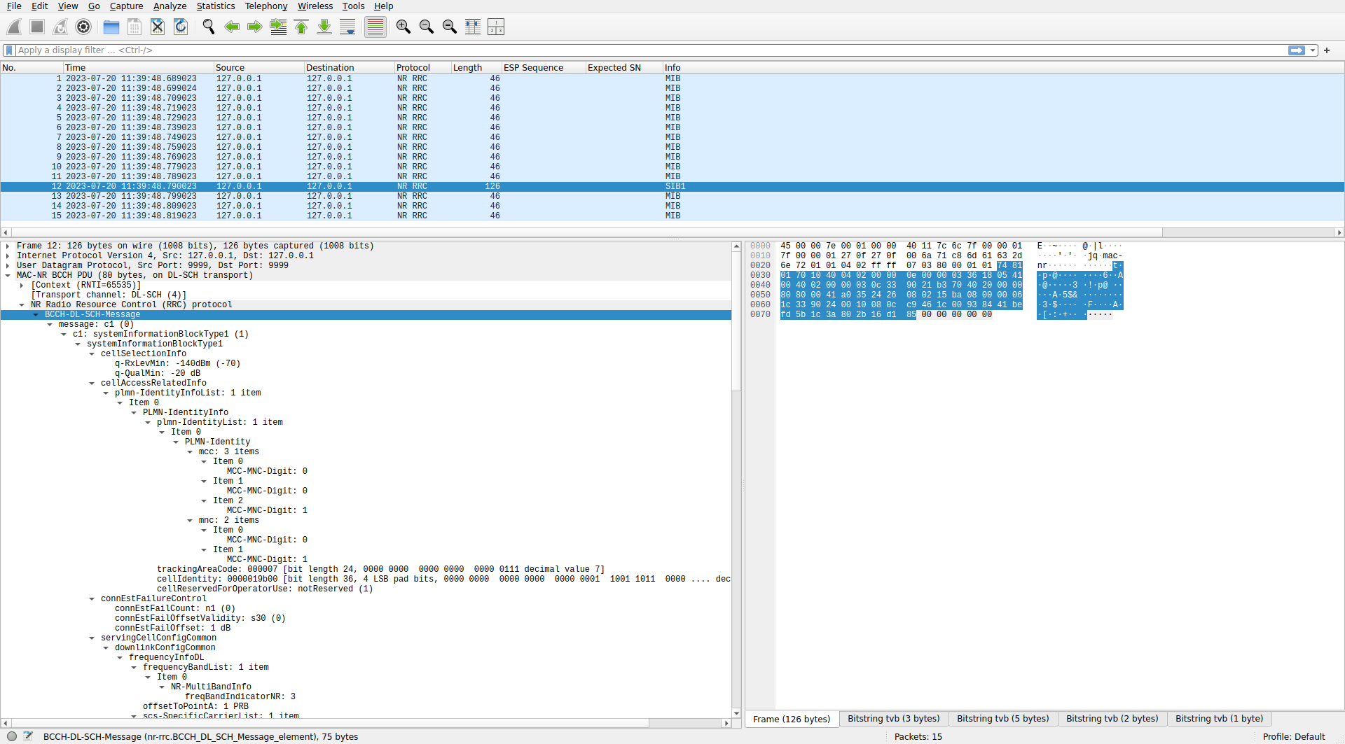
Since I am writing a PCAP file with the decoded data, the SIB1 can also be parsed in Wireshark. The following screenshots shows all the messages decoded from the recording, which are the MIB transmitted every 10 ms, and this SIB1 transmission.
Conclusions
Throughout this series of 5G posts I have used a short SigMF recording of an srsRAN gNB that does not have any attached UEs. The recording contains all the periodical signals that we would expect in a 5G downlink: the SSB, the CSI-RS, and the SIB1, which has a PDCCH and a PDSCH transmission. At this point I have decoded all the data signals and processed all the reference signals, so there is not much else to do with this file. If I continue this series about 5G, I will be moving on to some real world recordings, which will surely be much more varied and interesting.
Code and data
All the calculations and plots in this post are done in this Jupyter notebook. The SigMF recording can be found here.
Impressive work, as always!
Just a quick note: in order to speed up LDPC encoding and (especially) decoding, you can use a smaller sub-matrix by removing the latest rows and columns from the protograph (up to a certain limit).
The codes were constructed on purpose for this trick to work, although that is not clear at all from the standard.
This performance benefit will show up whenever the code rate is higher than the the “natural” one of the base graph. In your example R=0.37>0.2=1/5 (for base graph 2), this means that about half of the bits of the LDPC codeword can be ignored (in your figures, this would be the LLR=0 last half).
More info here (pages 4-5): https://www.nowpublishers.com/article/OpenAccessDownload/SIP-122
Thank you for the comment. Often there is a disconnect between the definitions in the 3GPP standards and the intentions and motivations about how best to use these algorithms. So it is great to have more insight.
Definitely the trick of speeding up an LDPC decoder by ignoring punctured parity bits that we do not need to solve for and part of the parity check equations is not unique to these 5G codes, but it is good to know that the 5G codes were designed with this specifically in mind. In the extreme example that I give in this post, the SNR is very good, so the only thing that the LDPC decoder needs to do is to solve for the information bits that were punctured. Already in the first decoder iteration this happens, but I wonder what is a minimal set of parity check equations that need to be used for this to happen.
For encoding I don’t think these kinds of tricks would work. All the parity bits that need to be transmitted over the air need to be computed. A smarter encoder would look at what rate matching is going to do and skip computing parity bits that would be punctured anyhow. In any case, encoding is usually much cheaper than decoding.
Actually Figure 4 in the paper you referenced makes quite clear how this works.
The parity check matrix for base graph 1 is of the form [[A B 0], [C D I]], where A is 4×22 (22 is the number of information bits), B is 4×4 and invertible, and I is the identity matrix. The first 4 parity bits can be efficiently encoded as y = B^{-1}Ax, where x are the 22 information bits. Since the remaining parity bits only appear once, in the I portion of the parity check matrix, the rows corresponding to parity bits that are punctured can be ignored on encoding. The remaining non-punctured parity bits can be encoded efficiently as the corresponding entries of z = Cx + Dy.
Likewise, for decoding the rows corresponding to punctured parity bits (except for the first 4 parity bits) can be ignored and removed from the Tanner graph.
In the above I have ignored lifting for simplicity, but the ideas are the same when lifting of the base graph is taken into account.