The Lunar GNSS Receiver Experiment (LuGRE) is a NASA and Italian Space Agency payload that flew in the Firefly Blue Ghost Mission 1 lunar lander. An overview of this experiment can be found in this presentation. The payload contains a Qascom GPS/Galileo L1 + L5 receiver capable of both real time positioning and raw IQ recording, and a 16 dBi high-gain antenna that was pointed towards Earth. For decades the GNSS community has been talking about using GNSS in the lunar environment, and LuGRE has been the first payload to actually demonstrate this concept.
The LuGRE payload ran a total of 25 times over the Blue Ghost mission duration, starting with a commissioning run on 2025-01-15 a few hours after launch and ending with a series of 9 runs on the lunar surface between 2025-01-03 (the day after the lunar landing) and 2025-01-16 (end of mission after lunar sunset). Back in October 15, the experiment data was published in Zenodo in the dataset Lunar GNSS Receiver Experiment (LuGRE) Mission Data. This dataset includes some short raw IQ recordings, as well as output from the real time GNSS receiver (raw observables, PVT, ephemeris and acquisition data). Since I have some professional background implementing high-sensitivity GNSS acquisition algorithms and I find this experiment quite interesting, I decided to do some data analysis, mainly of the raw IQ data.
The initial results of the experiment were presented on September 11 in the ION GNSS+ 2025 conference in a talk titled Initial Results of the Lunar GNSS Receiver Experiment (LuGRE). This talk is only available to registered ION attendees. As I don’t want to resort to my network to scrounge some ION paper credits (which is how proceedings are usually downloaded from the ION website), I haven’t seen anything about this talk besides the abstract. It is quite possible that something of what I will mention here was already presented in this talk. This is what we get as a society for not doing science in a completely public and open way. However, it’s interesting that this also makes my analysis less likely to be biased. I’ve just downloaded some raw IQ data and started looking at it with only basic context about the instrument that produced it and how it was run.
For a first analysis, I have implemented a high-sensitivity acquisition algorithm for the GPS L1 C/A signal in CUDA. I have run this on all the 20 L1 IQ recordings that are available. In this post I present the algorithm and the results.
Acquisition algorithm
Most of the parameters of the high-sensitivity acquisition algorithm are configurable. Here I will describe it with the nominal configuration intended to process the L1 recordings from LuGRE. The algorithm uses a coherent integration length of \(T = 20\, \mathrm{ms}\), matching the symbol duration of the GPS L1 C/A signal. This coherent integration is realized by performing a linear correlation with a replica with a duration of \(T\) and a signal window with a duration of \(2T\). This signal window is guaranteed to contain a full symbol. The linear correlation is implemented with a circular correlation done using FFTs. The FFT size is \(2 T f_s\), where \(f_s\) is the sample rate (8 Msps in the case of most LuGRE L1 recordings), and the replica of duration \(T\) is zero padded to a duration of \(2T\). Only the first \(T f_s\) samples of the IFFT are taken into account, since the full symbol contained in the signal window is guaranteed to start within the first \(T f_s\) samples. Note that the FFT size has only 2 and 5 as prime factors, so it can be implemented reasonably efficiently. An alternative implementation could choose an FFT size which is slightly larger than \(T f_s\) and zero pad both the signal and replica.
Doppler search is implemented by applying a circular shift to the FFT of the replica before performing the multiplication of the FFT of the signal and the complex conjugate of the replica. However, a circular shift by one position implements a frequency shift of \(1/(2T)\). For the nominal configuration we want a Doppler step of \(1/(4T)\). This is implemented by always working with two copies of the replica: one at baseband and one with an additional frequency shift of \(1/(4T)\).
Non-coherent integrations are done by working with signal windows that are advanced in steps of \(T\). Since the signal window duration is \(2T\), these windows overlap by 50%. A total of \(m = 14\) non-coherent integrations are used. This is because the total length of signal needed is \((m+1)T\), and most of the LuGRE IQ recordings have a duration of 300 ms (there is a single 200 ms recording which I’m ignoring, and a few longer recordings for which I’m only using the first 300 ms).
In order to avoid smearing of the correlation peak due to code Doppler, when the non-coherent integrations are added, a time shift of a few samples is applied to the integrations. This time shift is computed as the accumulated code Doppler at this integration, obtained from the carrier Doppler bin that is being computed, rounded to an integer number of samples. Note that code Doppler is ignored within each coherent integration of duration \(T\), since the replica is always generated with zero code Doppler. Non-zero code Doppler is only taken into account when stacking multiple integrations. Even though this time shift is only a few samples, there are edge effects to take into account. At the beginning and end of each integration, the time shift can require us to fetch samples from either the previous or the next integration.
A rule of thumb for acquisition sensitivity that is mentioned for instance in the Springer Handbook of Global Navigation Satellite Systems is that acquisition sensitivity, in terms of CN0 in dB·Hz, is given by\[13\,\mathrm{dB} – 10 \log_{10} T – 5 \log_{10} m.\]In our case this gives 24.3 dB. This rule of thumb is good as an initial guess, but it needs to be refined by taking into account the size of the search space and the presence of interference from other GNSS signals.
CUDA implementation
Initially I developed a prototype of this algorithm in a Jupyter notebook using CuPy to validate the algorithm. After that, I implemented the same algorithm in Rust using cudarc, cuFFT, and custom CUDA kernels in C++ that are compiled just-in-time for the required acquisition parameters. I have made a new Rust crate called gnss-dsp with the intention that of adding more GNSS signal processing algorithms to that crate in the future. The crate uses PyO3 and Maturin for Python bindings, and it is also available as a gnss-dsp Python package. The Python package contains some convenient Python CLI scripts that run the acquisition and generate plots with Matplotlib.
The CUDA implementation of the algorithm works as follows. First, \((m+1) T f_s\) signal samples are copied to the GPU. The FFTs of the \(m\) window signals are computed with a single cuFFT call that performs FFTs with 50% overlap. The results are stored in the GPU, so they can be reused to acquire with different PRNs.
The acquisition works iteratively on multiple PRNs. How many PRNs can be used in a single call is limited by host memory, since the results (which are a full Doppler-delay map of \(T f_s\) samples in the delay dimension and \(4 T \Delta f\) Doppler bins in the Doppler dimension, where \(\Delta f\) is the total Doppler range to cover) for all the PRNs in each call are stored in an array in host memory.
For each PRN, a baseband replica of length \(T f_s\) samples is computed. This baseband replica is then shifted in frequency to generate the other \(k – 1\) replicas, where \(k\) is the Doppler oversampling factor, which gives a Doppler step of \(1/(2kT)\). By default, \(k = 2\), so only another replica is generated. The FFT of all these \(k\) replicas is then computed with cuFFT. In order to make circular shifting of the replica more efficient, two repetitions of each replica are stored consecutively in GPU memory. This is achieved by performing a device-to-device memory copy after the FFT is finished.
Circular shifts that are used to perform Doppler shifts by multiples of \(1/(2T)\) are evaluated in Doppler blocks, which compute \(r\) of these circular shifts at once. Since intermediate results for all the \(kr\) Doppler bins in the Doppler block are stored in GPU memory, the size of a Doppler block is limited by GPU memory. For each Doppler block, a signal_replica_products CUDA kernel is launched to compute the product of the all the \(m\) signal window FFTs times the complex conjugates of all the \(k\) replica FFTs for all the \(r\) circular shifts in the Doppler block. Because two consecutive copies of each replica FFT are stored in GPU memory, the circular shift is implemented simply as an address offset when reading the replica. After the signal_replica_products kernel finishes, a cuFFT call is done to compute the IFFTs for all \(mkr\) products.
The final step is the non-coherent accumulations. An offset in samples (as a floating point number) per non-coherent integration is computed in terms of the carrier Doppler. The same value is used for all the Doppler bins in the Doppler block, since their difference in accumulated code Doppler is quite small for typical Doppler block sizes. A noncoherent_accumulate CUDA kernel is called to compute the non-coherent accumulations. For each of the \(kr\) outputs in this Doppler block, and for each of the \(m\) integrations in each output, the kernel computes the complex magnitude squared of the IFFTs and adds each of the \(m\) integrations, writing the result of the accumulation to the results array in GPU memory.
After all the Doppler blocks corresponding to the required Doppler range are computed, the acquisition algorithm performs a GPU to host memory copy to copy the results for this PRN to the host array that contains the results for all the PRNs in the call. It then proceeds with the remaining PRNs in the list of PRNs to acquire.
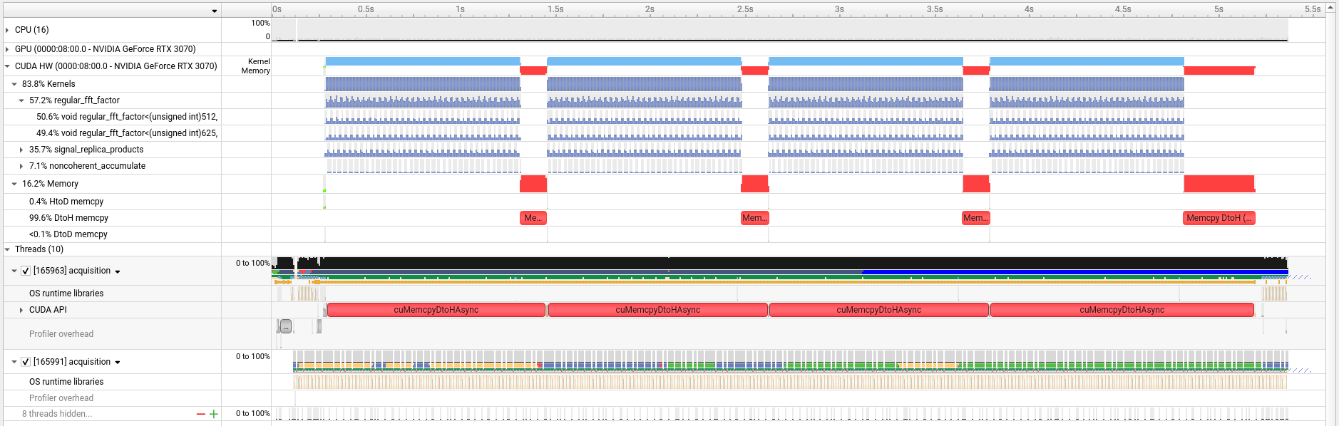
A simple acquisition benchmark example is included in gnss-dsp. It acquires 4 PRNs in a single call using a Doppler range of -10 kHz to +10 kHz and a Doppler block size of 8 circular shifts. This takes about 4.9 seconds to run on an RTX 3070 and uses 2.9 GiB of GPU memory.
The following figure shows profiling results for the acquisition benchmark example in nsys-ui. We can see the four computes for each PRN followed by the device to host copy of the results. I don’t know why the last device to host copies takes much longer, since all the copies have the same size. I have seen varying levels of throughput for these copies in multiple runs of the same benchmark.
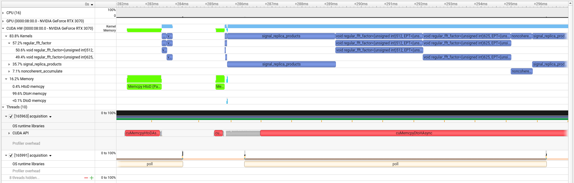
The beginning of the acquisition benchmark looks like this. First all the signal samples are copied to the GPU. Then the signal FFTs are computed by two calls to cuFFT kernels. When computing FFTs of size 320000, there is always one kernel to perform the factor 512 of the decomposition of the FFT size using radix 8 and another one to perform the factor 625 using radix 5. Then there is some time in which the host is computing the replicas. These are then copied to the GPU and their FFTs are computed, followed by the device to device copy used to duplicate the FFTs in GPU memory. Then the loop over Doppler blocks begins. This is always formed by the signal_replica_products kernel, the two kernels implementing the IFFTs, and the noncoherent_accumulate kernel.
Acquisition results processing
For each PRN, the acquisition algorithm returns an array corresponding to the cross ambiguity function (CAF) of the signal and the replica generated for that PRN. In the Doppler dimension the array has a resolution of \(1/(2kT)\) (by default \(k = 2\)) and it covers the specified Doppler range. In the time dimension the array has a resolution of one sample and it covers the delay range between zero and \(T\).
The entry where this array has maximum value is searched to determine the Doppler and delay corresponding to the acquisition result. By default this searches over the whole array, but it is possible to limit the search along the time dimension to a particular range, which is useful in some cases that will be presented below.
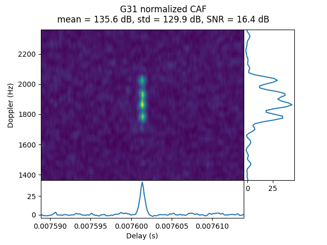
The mean and the standard deviation of the array are computed. Acquisition SNR is measured by subtracting the mean and normalizing by dividing by the standard deviation. Note that in the case of a strong signal, the mean is positively biased by the correlation peak. However, this algorithm is mostly intended for weaker signals, for which this bias is negligible.
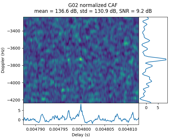
The following plot shows the CAF for a simulated signal with 24 dB·Hz of CN0. The plot has been obtained by running
gnss-acquisition-simulation --plots-dir /tmp/plots --cn0 24
The plots show the normalized SNR in linear units, but the title of the plot gives values in dB. In this case the delay of the simulated signals is zero seconds. However, for weak signals the correlation peak can appear at another multiple of the code period close to the symbol edge (19 ms in this case) because of the random contribution of noise, particularly if the simulated signal has few symbol changes.

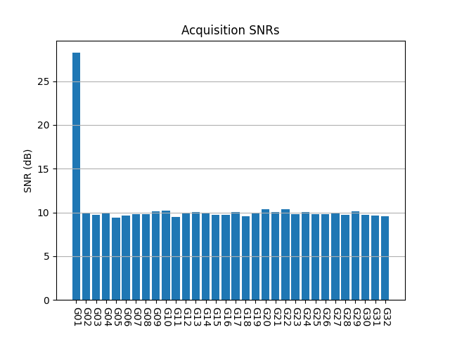
In this simulation the signal is only G01 plus AWGN. Other PRNs will also show what appears to be a small correlation peak at a random location, but this is just because of the random contribution of AWGN, because the search space is rather large (20 ms times 20 kHz in this case).
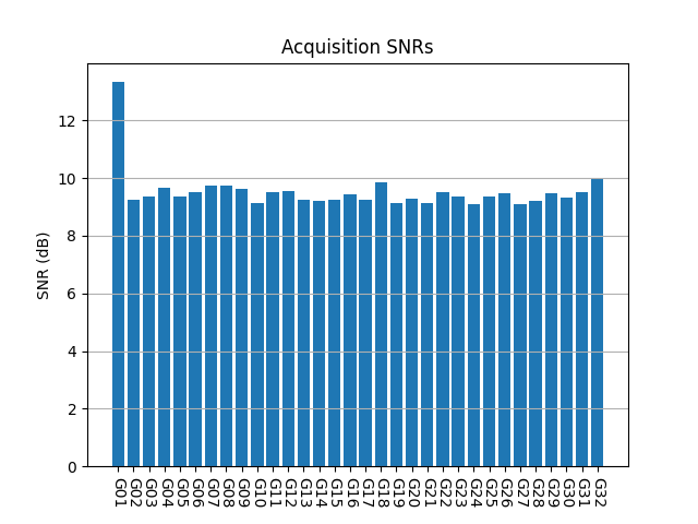
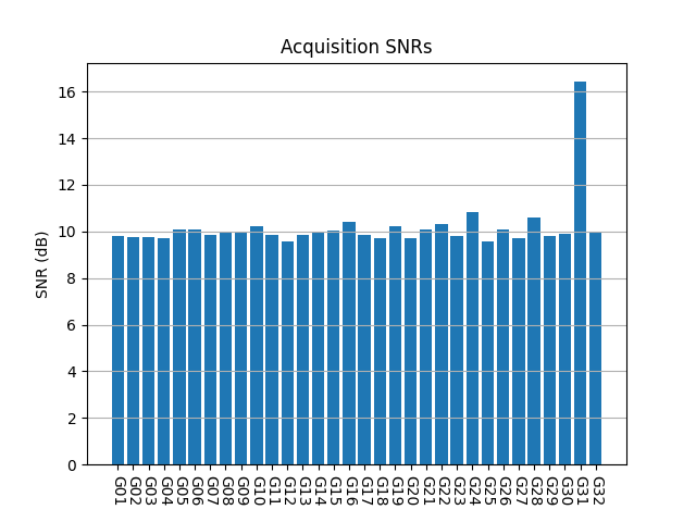
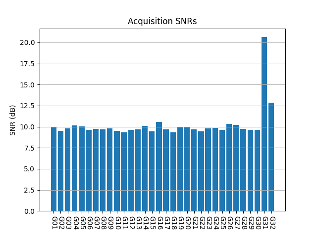
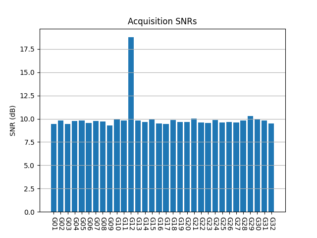
The following plot shows the acquisition SNRs obtained for all the PRNs in this simulation. We can see that PRNs that are not present have an SNR around 9 to 10 dB. G01, which is the only one present, has an SNR around 13 dB, so it can be detected reliably. Note that in this case the delay and Doppler of G01 are perfectly aligned with one of the CAF bins that are computed, so there are no correlation losses because of residual delay or frequency error.
A problem with the GPS L1 C/A code is that the cross correlation between different PRNs is relatively high, specially if we also consider frequency offsets which are integer multiples of 1 kHz. The consequence of this for high-sensitivity acquisition algorithms is that if there is a relatively strong signal from one PRN, there will be false acquisitions for PRNs which are not present due to this cross correlation. The Doppler frequency of these false acquisitions is typically close to the Doppler frequency of the strong PRN plus an integer multiple of 1 kHz.
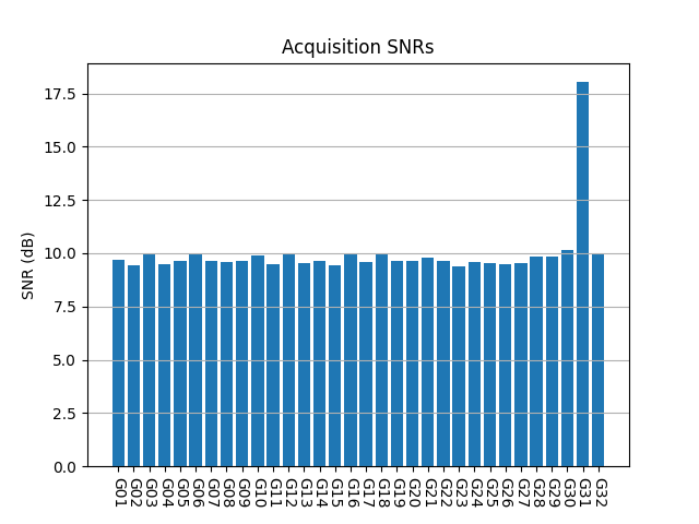
A demonstration of this effect is obtained by performing the same simulation but with a CN0 of 40 dB·Hz for G01. The acquisition SNRs for PRNs that are not present are slightly higher than before.
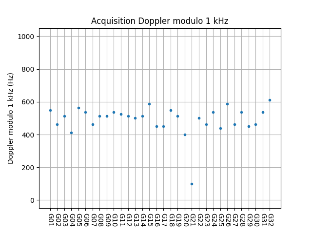
If we plot the acquisition Doppler modulo 1 kHz, we can see that most PRNs have values that are close to 0, which is the Doppler frequency of G01. This means that the correlation peaks found by the acquisition algorithm are actually caused by cross correlation with the G01 signal.

This kind of plot is quite useful to judge if cross correlation effects are happening. In the LuGRE data we will see that this does not happen, since we don’t have signals that are strong enough.
Results obtained with the LuGRE data
I have run the acquisition algorithm on all the LuGRE L1 recordings (except IQS_L1_20250119_045211_200MS_T_OP5_0, which is only 200 ms long) using a Doppler search range from -25 kHz to 25 kHz. The characteristics of each recording are listed in an OPTABLE.csv file included in the dataset.
Here I show only the recordings in which some GPS L1 C/A signals were detected by this acquisition.
IQS_L1_20250116_013117_400MS_C_OP2_0
OP2 was a commissioning run done at 25.25 Earth radii distance. Two reasonably strong signals are detected.

However, when we look at the CAF of these two PRNs, we see that there is a huge spread in Doppler. I investigate this in more detail in a section below.
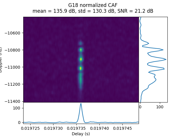

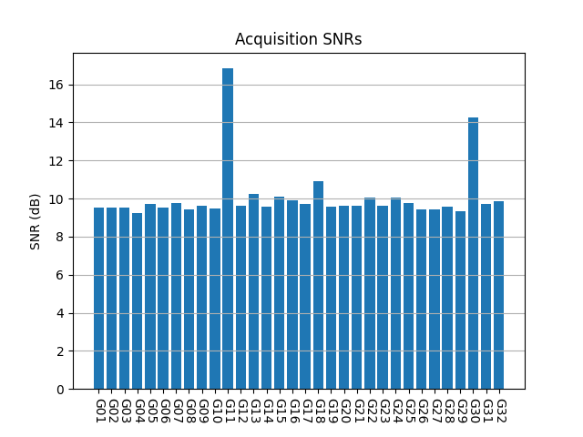
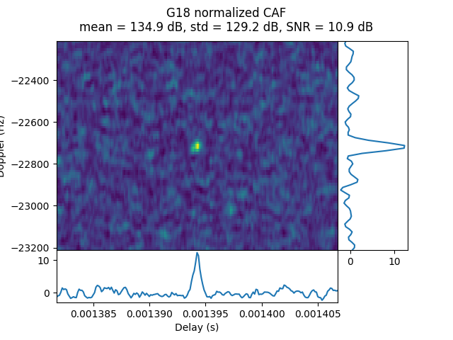
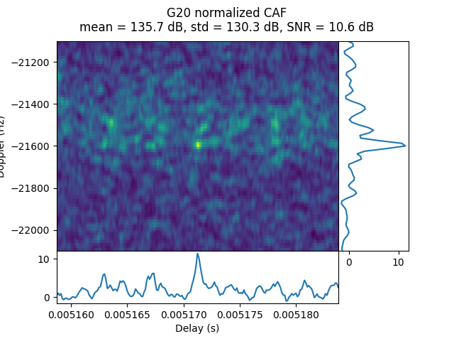
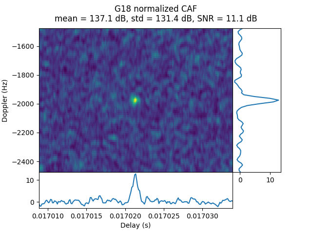
IQS_L1_20250203_091340_400MS_T_OP17_0
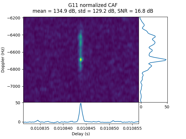
OP17 was done during the transfer orbit at a distance of 44.91 Earth radii. G11, G31, and possibly G18 are detected.
In the CAF of the two stronger signals we can see a Doppler spread effect.
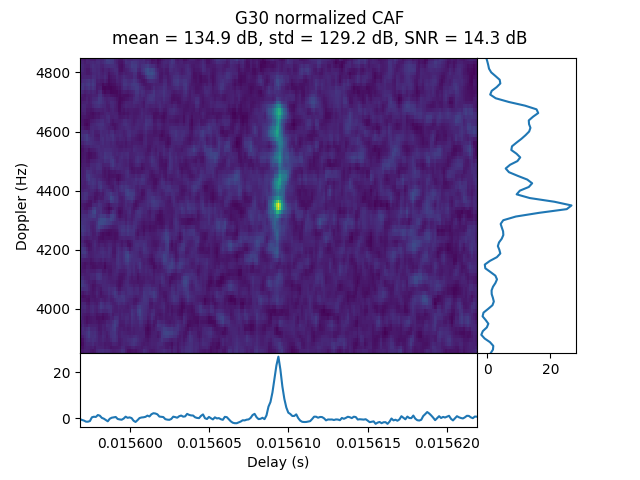
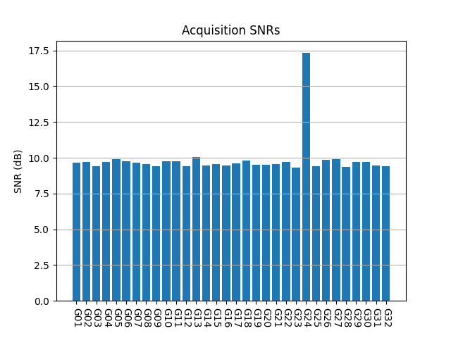
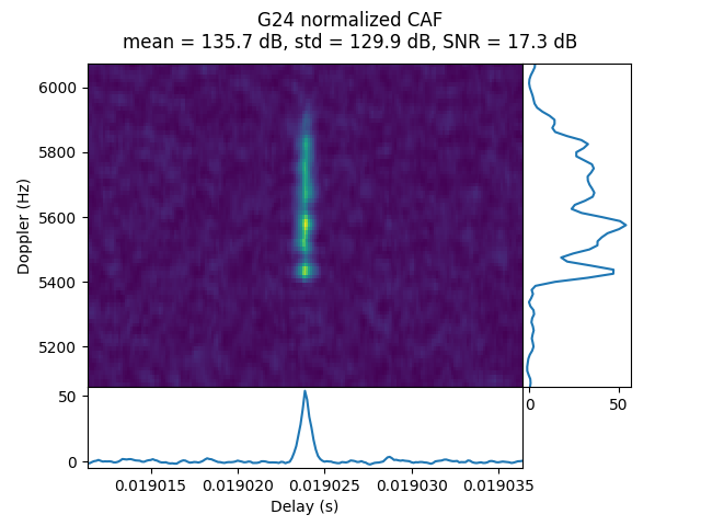
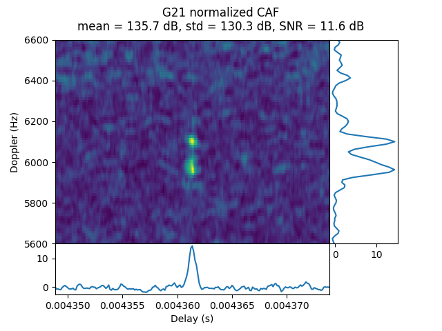
IQS_L1_20250207_232901_600MS_T_OP21_0
OP21 was done during the transfer orbit at 32.63 Earth radii distance. Only G24 is detected.
In the CAF we see the usual frequency spread.
IQS_L1_20250212_034755_400MS_T_OP22_0
OP22 was done during the transfer orbit at a distance of 52.92 Earth radii. Only G31 is detected. Its CAF shows frequency spread.
IQS_L1_20250214_045853_400MS_L_OP23_0
OP23 was done in lunar orbit at a distance of 61.19 Earth radii. This is an interesting dataset. Looking at the plot of SNRs it is not obvious that there are any detected signals, although the SNRs are all slightly higher than usual. The plot of Doppler modulo 1 kHz shows all the PRNs except one inside a band.

What happens in this recording is that G21 is present, although there is some Doppler spread.
Other PRNs show a horizontal band in the CAF plot. This is probably caused by interference. It also happens in other datasets. There is weak CW interference around -420 kHz and -400 kHz in this and other datasets. Perhaps this is what causes this interference.
IQS_L1_20250224_120449_300MS_L_OP32_0
OP32 was done in lunar orbit at a distance of 58.93 Earth radii. Only G06 is detected, with a rather weak signal.

The CAF for G06 doesn’t show any frequency spread, but maybe that is just because the signal is weak and the spread is below the noise floor.

IQS_L1_20250304_070323_300MS_S_OP40_0
OP40 was done from the lunar surface at a distance of 56.25 Earth radii. G25 is detected with a reasonably strong signal, and perhaps G18 is present with a weak signal.

In the CAF of G25 we do not see any frequency spreading, and this signal is strong enough that the spreading would show up if it was present.

IQS_L1_20250314_124717_500MS_S_OP74_0
OP74 was done from the lunar surface at a distance of 61.9 Earth radii. Only G31 is detected, but it has a rather strong signal. There is some Doppler spread in the CAF, but it is narrower than in other recordings.

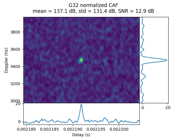
IQS_L1_20250315_130727_2000MS_S_OP76_0
OP76 was done from the lunar surface at a distance of 62.2 Earth radii. Unlike most other recordings, it is 2 seconds long. G31 and G32 are detected. Their CAFs do not show any Doppler spread.

IQS_L1_20250316_191504_300MS_S_OP77_1
OP77_1 was done from the lunar surface at a distance of 62.44 Earth radii. The acquisition SNR shows weak signals for G06 and G14. The signals actually have large Doppler spread in their CAFs, which lowers the effective SNR. The spread patterns are noticeably different unlike in other recordings.


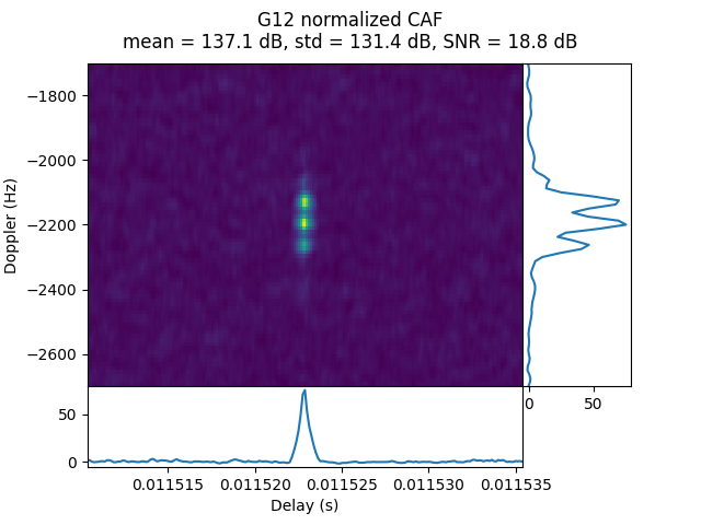
IQS_L1_20250316_220402_300MS_S_OP78_0
OP78_0 was done from lunar surface at a distance of 62.45 Earth radii. G12 has a strong signal, with some Doppler spread.
IQS_L1_20250316_221128_300MS_S_OP78_1
OP78_1 was done just 10 minutes after OP78_0, so the results are similar. G12 is present with a strong signal. In this case the Doppler spread is much larger than in OP78_0.


Doppler spread analysis
We have seen that in most of the recordings the CAFs show a large amount of Doppler spread. To investigate this, I have processed OP78_1 again with some specific parameters to make a video that shows how the CAF evolves over time. These parameters are:
- Coherent integration length: 10 ms
- Only one non-coherent integration
- Doppler oversampling: 8 (gives a frequency resolution of 6.25 Hz)
- Rather than finding the maximum CAF peak over a window of 20 ms (twice the coherent integration length), the CAF is restricted to the first 1 ms window
- The file is processed in steps of 1 ms to obtain each frame of the video
These processing parameters give us a view of how the CAF evolves over time in 1 ms steps. I have chosen OP78_1 for this analysis because it has a relatively strong signal with large Doppler spread, and because the receiver was “stationary” on the lunar surface.
The video of the CAF of G12 in OP78_1 is shown here.
We can see three effects. First, the Doppler frequency moves down at a roughly constant rate throughout the recording. Second, we can sometimes see how the CAF peak splits into two peaks that are at ±100 Hz offset of where they should be. This effect is fully expected. It happens when the 10 ms coherent integration contains a symbol change. Third, there is significant fading in the signal. When the CAF peak splits, the power will be divided equally between the two peaks, but we can also see large drops in signal power in other moments.
For comparison, this is how a simulated signal with a constant Doppler of 3 kHz and 40 dB·Hz CN0 looks like when processed with the same parameters.
The conclusion is that the Doppler frequency of the signal is changing throughout the recording because the receiver clock drift (frequency reference) is changing. A change of 500 Hz over 280 ms is too much to be explained by line-of-sight dynamics, specially since I have picked a recording where the receiver is on the lunar surface. This change corresponds to approximately 300 ppb, so the drift is on the order of 1 ppm/s. This is quite a lot.
If I had to guess the cause of this problem, I would say that it is a thermal effect that happens when the receiver starts working. I am quite surprised that most of the recordings have this problem. This issue should have been detected and fixed while testing the instrument on ground before launch.
I haven’t looked into how this problem impacts the real time positioning data. My guess is that if this is a thermal effect, it will only last for the first few minutes until things settle. Since each real time positioning session last a few hours, the impact would be minimal.
Since IQ recordings are very short, they are completely affected by this issue even if it is a transient (except for OP40_0 and OP76_0, which do not present this problem at all). This is a pity. It is not that the data is completely bad, but a drift on the order of 1.5 kHz/s is too large for typical GNSS receiver algorithms (this corresponds to an acceleration of 29 g), so the drift would need to be estimated and corrected before trying to use these recordings to test algorithm performance.
Analysis of OP76_0
Since OP76_0 is 2 seconds long and it does not have the frequency drift problem, it is without any doubt the best recording in this dataset. I have made a video of the CAF of G31 in this recording using the same processing parameters as in the previous section.
Since this video spans 2 seconds of data, we can see how the code delay and Doppler slowly change throughout the recording. The fading is also quite noticeable. I am somewhat impressed that this relatively strong signal has so much fading. Perhaps there is a contribution of multipath due to a reflection on the lunar surface. However, the landing site of Blue Ghost Mission 1 has a latitude of 18.6º, which means that the Earth would be quite high in the sky as seen from the Moon. This should make ground reflections less likely.
Conclusions
In this post I have presented a CUDA high-sensitivity acquisition algorithm for GPS L1 C/A that can also be repurposed to compute the evolution of the CAF over time (in the form of a Delay-Doppler map, which is commonly used in GNSS reflectometry). I have run this over the LuGRE L1 recordings and observed that out of 19 recordings, signals can only be detected in 12 of them. The number of satellites in each of these 12 recordings ranges between 1 and 3.
There is a receiver frequency drift problem in most of the recordings. This affects the sensitivity of the acquisition algorithm, so it is possible that some weaker signals have not been detected because of this.
I have not looked into the geometry of the detected satellites. I expect that those that have strong signals have the receiver in the main beam of their antenna. This means that, as seen from the receiver, the satellite is illuminating the Earth from “behind”, but still there is direct line of sight to it. Looking at the geometry in Figure 5 in this paper, we see that the GPS Block IIF antenna is design to illuminate up to 23º off nadir, while the edge of Earth is at 13.8º off nadir. Since the portion of the area of the sphere that is occupied by a spherical cap defined by a spherical cone with aperture \(2\varphi\) is \((1- \cos \varphi)/2\), we see that taking into account blockage by the Earth, the fraction of the celestial sphere illuminated by a single satellite is\[\frac{\cos 13.8º – \cos 23º}{2} \approx 0.0343.\]This means that assuming that the GPS satellite positions are randomly and uniformly distributed over the celestial sphere (which is not really true, but it is useful to obtain a ballpark approximation) and that the constellation has 32 satellites, on average only 1.1 satellites illuminate with their main beam a given point that is far enough from Earth. This intuition roughly matches what we have seen in this dataset, and it limits the feasibility of using GNSS for navigation in the lunar environment.
Code and data
The acquisition algorithm used in this post is implemented in the gnss-dsp Rust/Python package. There is an additional repository called lugre that contains the scripts that automate the data processing. The data was published in the Zendo dataset Lunar GNSS Receiver Experiment (LuGRE) Mission Data by the LuGRE team.
Hey, loved the work here! I am also playing with this dataset at the moment and was interested in seeing the videos of how the Doppler spread is moving in time, however, I see that the videos do not work. Could you please upload them again?
Also, for the satellites with strong signals, did you also try to coherently combine not for a 10 or 20 ms but about 2 ms of coherent and about 150 (maybe less) non-coherent combinations? It should (and my simulations did) show some robustness to these effects. However, even with this being the case, this seems like quite an interesting effect that requires further attention!
I hope that they also share even longer acquisition samples for us to have tracking over a longer interval for further analysis.
Also, what was the lowest C/N0 you were able to capture in your simulations?
I haven’t gone through the full exercise of doing Monte Carlo simulations to determine a suitable threshold for a given probability of acquisition and then computing the acquisition probability versus CN0 based on that. I expect that the ballpark formula that I gave (which says 24 dB·Hz) will be within a few dB of the real performance.
If the videos aren’t playing correctly for you, that is most likely a browser issue. Uploading them again won’t fix it. You can download the videos (the URLs are in the page HTML source code) and play them locally. Or clone the repository and generate them locally.
I didn’t try shorter coherent integrations. I know that the stronger satellites will still be detectable and that this will make the frequency drift less evident, but that is not the point.
I think this is the full data release of all the data that was recorded during the mission. I don’t think there are any longer IQ recordings.