This year I submitted a track of challenges called “Not-LoRa” to the GRCon 2024 Capture The Flag. The idea driving this challenge was to take some analog voice signals and apply chirp spread spectrum modulation to them. Solving the challenge would require the participants to identify the chirp parameters and dechirp the signal. This idea also provided the possibility of hiding weak signals that are below the noise floor until they are dechirped, which is a good way to add harder flags. This blog post is an in-depth explanation of the challenge. I have put the materials for this challenge in this Github repository.
To give participants a context they might already be familiar with, I took the chirp spread spectrum parameters from several common LoRa modulations. These ended up being 125 kHz SF9, SF11 and SF7. LoRa is somewhat popular within the open source SDR community, and often there are LoRa challenges or talks in GRCon. This year was no exception, with a Meshtastic packet in the Signal Identification 7 challenge, and talks about gr-lora_sdr and Meshtastic_SDR.
It’s not a secret that I don’t like LoRa and its popularity very much. This is rooted in the times where it was a proprietary and patented protocol, and the reverse-engineered SDR implementations were not very good. I just felt that it wasn’t a good idea to include LoRa so pervasively into the open source and amateur radio spheres, because the status of the protocol was completely opposite to what these communities stand for. Also, from the technical point of view, LoRa’s weak SNR performance is not at all impressive (just calculate the Eb/N0 that it needs to decode). The situation has perhaps changed somewhat over the last few years. Now SDR implementations such as gr-lora_sdr are certainly very good, and I think more technical documentation about the PHY is available (though don’t quote me on that, because I can’t find it). I also reckon that LoRa’s strong points are co-channel interference resistance and the fact that it performs much better than GFSK tranceivers in the same price range. In any case, doing a challenge track heavily inspired by LoRa was also a way of making some fun of myself.
The challenge track has a single SigMF recording and five flags that can be solved in any order. The challenges are given without any additional explanation, since the first flag, which is very easy to get, gives some more information. The .sigmf-meta file contains the following information. The frequency is yet another reference to the band where LoRa typically operates. The "core:hw" is a joke, but it is also intended to convey the idea that the signals are generated in software, so all sorts of tricks can be expected.
{
    "global": {
        "core:author": "Daniel Est\u00e9vez <daniel@destevez.net>",
        "core:datatype": "ci16_le",
        "core:description": "Not-LoRa (GRCon24 CTF challenge)",
        "core:hw": "No hardware was harmed in the making of this challenge",
        "core:license": "https://creativecommons.org/licenses/by/4.0/",
        "core:recorder": "GNU Radio 3.10",
        "core:sample_rate": 525000,
        "core:sha512": "5b50d6c9e799f6acc81d2d3589f681f4380d772d8d19d9b3e38a90de2c5655aa08e77dde9e217760863493f524dae14d4cc891b1a7aadc9276a0f56524ad2a7d",
        "core:version": "1.0.0"
    },
    "captures": [
        {
            "core:frequency": 915000000,
            "core:sample_start": 0
        }
    ],
    "annotations": []
}
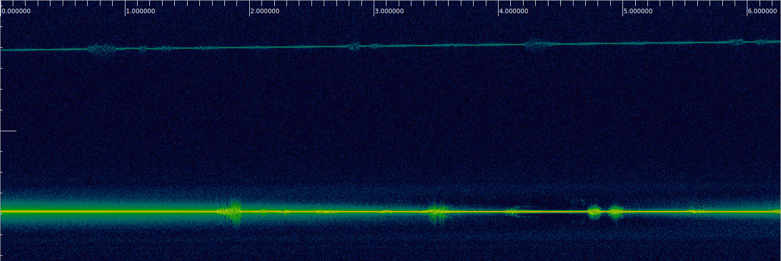
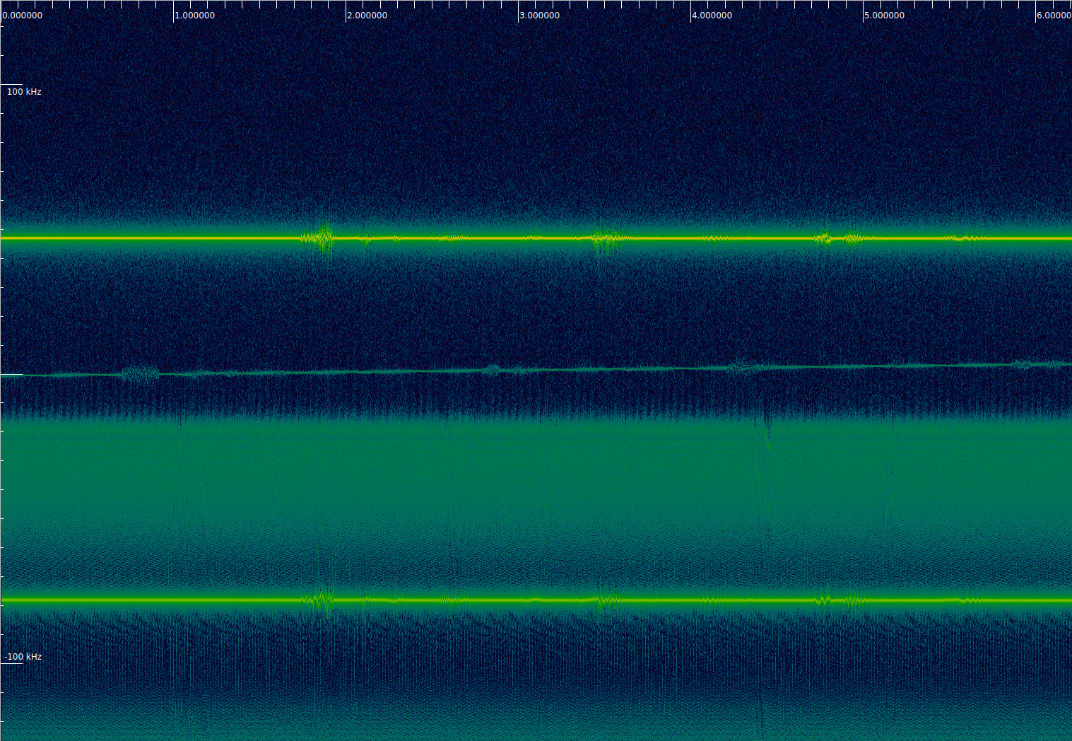
A look to the recording with reasonable FFT size and zoom parameters in Inspectrum reveals multiple chirped signals.
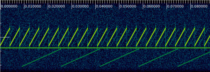
There are in fact four signals visible in this waterfall, and each of them contains a different flag. One signal is not chirped and might be mistaken by a CW carrier with this FFT size, but as we will shortly see, it is a plain narrowband FM voice signal. The other three signals are chirped. Two of them stand out, and have noticeably different chirp rates (the difference is a factor of 4). The other signal is weaker and is placed between the chirps of the signal in the centre of the waterfall. It has the same chirp rate and bandwidth but a different chirp phase. Some participants might have mistaken this weaker signal for some kind of artifact (perhaps multipath) of the stronger signal, but it is in fact a different signal. The game here is that two signals with the same chirp parameters and frequency can be separated as long as their chirps are out of phase, even if they have largely different SNRs.
A different FFT size and zoom shows that the signal that is not chirped is just a narrowband FM voice signal. It says “None of the signals in this challenge are LoRa”, and then it gives flag 1, which is a series of numbers (just like the rest of the flags in this track).
This flag is intended to be very easy (everyone playing the CTF should be able to get it!) and to introduce the challenge. It gets participants into thinking about LoRa, but discourages from attempting to throw in a LoRa receiver to try to solve the challenge (those more familiar with LoRa might have already realized that a LoRa receiver won’t work, because LoRa packets include a syncword that is formed by downchirps, while there are no downchirps in this recording).
It is easy to measure (in Inspectrum, for instance) that the bandwidth of the chirped signals is around 125 kHz, and their chirp rate is 4.096 ms and 16.384 ms. This might ring some bells and point to LoRa SF9 and SF11 respectively, which use these chirp parameters. The key formula here is that the LoRa chirp rate is \(2^{\mathrm{SF}}/{\mathrm{BW}}\), where SF is the spreading factor (an integer between 7 and 12) and BW is the bandwidth (the following bandwidths are supported: 7.8 kHz, 10.4 kHz, 15.6 kHz, 20.8 kHz, 31.25 kHz, 41.7k Hz, 62.5 kHz, 125 kHz, 250 kHz, 500 kHz). A good way to remember this formula is to know that the LoRa demodulator works internally with a sample rate equal to the bandwidth (I will explain why later on) and performs an FFT to demodulate each symbol. To implement this FFT efficiently, the symbol duration is constrained to a number of samples that is a power of 2, and the allowable powers of 2 are between \(2^7\) to \(2^{12}\), giving the different spreading factors.
Knowing the chirp rate, a tempting idea is to perform dechirping and see what happens, but before doing that we can even understand more properties about our signals if we look more closely in Inspectrum. In some parts of the recording, with the appropriate FFT size and zoom, it is apparent that the upper strong signal wobbles in frequency. This suggests frequency modulation, and in fact flag 1 being a narrowband FM voice signal was intended to point participants in the right direction for some of the other flags. This chirped signal is also narrowband FM voice, albeit with LoRa-like chirp spread spectrum on top of it.

The lower signal seems to be fading in and out. This suggests AM modulation. In fact this signal is AM modulated with a voice signal. When designing this challenge, my intended solution was to dechirp this signal too. I put AM instead of FM just for the sake of variety. However, when beta testing the CTF challenge, Clayton found a shortcut that I didn’t expected (but which was obvious in hindsight). It’s not even necessary to dechirp this AM signal. Just pointing a regular AM receiver somewhere inside the 125 kHz signal bandwidth will give you understandable audio, as long as the bandwidth of the AM receiver is large enough. This is because the SNR is relatively good. For a weaker signal you would have needed to dechirp to get processing gain. Perhaps Clayton realized this trick because one of its own challenges, “Nothing but noise”, involved a recording that at first glance was only AWGN, but where a chunk of approximately 100 kHz had been AM modulated with voice in a way that it was rather inconspicuous but such that putting an AM demodulator anywhere in this chunk would give you some marginally understandable speech. This AM signal gives flag 4. The shortcut is the reason why this flag gives lower points than the other ones. The audio obtained in this way, with the widest AM receiver allowed by GQRX, is shown here. It isn’t pretty, but the flag can be copied easily.
Now let us think about dechirping the FM signal, which contains flag 2. Since we know the chirp parameters, we can generate the same chirp waveform and perform a multiply conjugate operation to remove the chirps from the signal. I’ll call this clean chirp waveform the “local chirp”, since it’s generated locally by the receiver to perform dechirping. Unless we adjust the chirp phase of the local chirp very precisely to the chirp phase of the received signal, we will get a nasty effect. If the two chirps are somewhat out of phase, one of them will reach the higher edge of the bandwidth and wrap around to the lower edge before the other. During this period of time, the frequency difference of the two chirps will be ±125 kHz more than the rest of the time (the sign depends on whether the received signal or the local chirp is leading). If the local chirp is aligned in chirp phase better to the received signal, the length of this period will be shorter, reaching zero when the two signals are perfectly aligned. I had mentioned this effect in an old post about CODAR, which is a chirped radar used for ocean wave sensing.
If we look at the spectrum of the dechirped signal, we will see two copies of the signal separated by 125 kHz. The relative power of the signals tells us how well the local chirp phase is aligned to the received signal. With perfect alignment, one of the two copies of the signal disappears. This gives a way to align the chirp phase by hand. What is actually happening is that the dechirped signal jumps between these two frequencies in each chirp period. If the local chirp alignment is better, the signal spends less time on one of the two frequencies, and more signal power is concentrated in the other frequency.
However, for an audio FM signal these frequency jumps are really nasty. Unless the chirp phase is aligned very well, the jumps cause a strong humming noise in the audio, which makes it impossible to understand the speech. The reason is that FM is really sensitive to these jumps. During the period when the signal has gone 125 kHz away, the FM receiver sees only noise, so its output goes haywire because the frequency measured on the noise is random. For the SF9 signal this causes strong pulses at the audio output with a rate of 244 Hz. Other types of modulation such as AM and SSB are not too sensitive to these jumps. During the jump, the receiver sees noise which is weaker than the signal, and the jump is brief enough that the AGC doesn’t kick in, so there is very little effect in the audio (as an interesting side note, I read somewhere that Leif Asbrink SM5BSZ did some experiments by switching at kHz rate an SSB system between TX and RX in order to listen to his own echos on the aurora, and the transmitted audio was still quite readable).
To be fair, I should mention that the behaviour of an FM receiver when the signal briefly jumps 125 kHz away really depends on the demodulator algorithm that is used. The above explanation refers to the quadrature demodulation algorithm, which is commonly used in SDR. A PLL-based receiver might not be so sensitive, especially if the error discriminant is scaled with the signal amplitude. Likewise, a receiver that converts FM into AM by passing the signal through a filter that has an amplitude versus frequency slope will not be affected so much by these jumps.
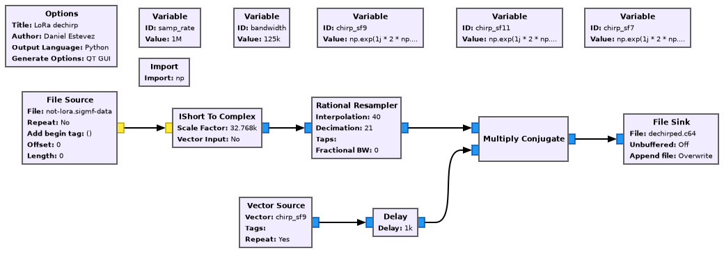
The dechirp can be done with the following GNU Radio flowgraph. For simplicity, I’m resampling the recording from 525 ksps to 1 Msps, because this gives an integer number of samples per chirp. A single local chirp is calculated with a Numpy expression in a Variable and repeated forever with a Vector Source. The Delay block can be used to adjust the phase of the local chirp with respect to the received signal.
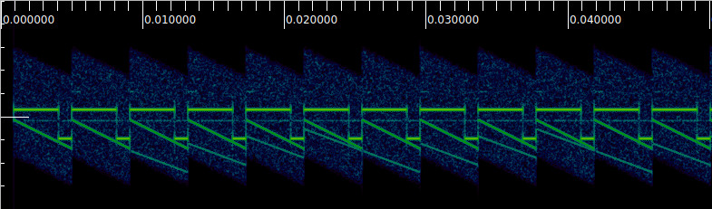
When the local chip is significantly out of phase with the received signal, we can see two copies of the same FM signal, separated by 125 kHz. One of the copies is weaker.
With a different time resolution it is apparent that the signal keeps jumping back and forth between these two frequencies. The time spent on the second frequency is proportional to how much the received signal and local chirp are out of phase.
The results with this misalignment are not very good. The audio of the FM receiver in GQRX can be heard here. It is almost impossible to copy the flag.
With much better alignment between the received signal and the local chirp, the signal now looks like this. It only spends a very brief time in the second frequency.
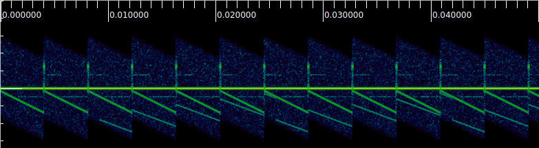
The quality of the audio is now much better, and the flag can be copied, but there is still that annoying buzz.
In the CTF solutions walkthrough, Clayton mentioned a trick to avoid the 125 kHz jumps when the receive signal and local chirp are out of phase. The trick is essentially to work at 125 ksps. In this way, the two signals 125 kHz apart alias to the same frequency, so the is no jump. There are two ways to implement this trick. One is to downconvert the received signal and decimate it to 125 ksps, and then perform dechirping at 125 ksps, and the other way is to perform dechirping at the original sample rate and decimate the result to 125 ksps. The important thing is that we look at the final result at 125 ksps.
There is something important to note: regardless of the method, a lowpass filter with slightly more than 125 kHz (two-sided) bandwidth needs to be used with the decimation to 125 ksps. When decimating, the common thing to do is to use an anti-alias filter whose bandwidth is slightly narrower than the output sample rate. In this situation, using a filter slightly wider than 125 kHz, which actually produces some aliasing, is the correct thing to do. The reason is that in the first approach, the bandwidth occupied by the chirped received signal is slightly more than 125 kHz. If we filter it with a bandwidth narrower than 125 kHz, we will be chopping off the edges of the signal, and so the dechirped signal will have some periodic fades due to the chopped off edges. In the second approach it is even more obvious that we need a filter wider than 125 kHz. Since the dechirped signal jumps between two frequencies 125 kHz apart, a filter narrower than this cannot possibly let the two frequencies through.
This trick of working at 125 ksps is also how a LoRa receiver typically works. In LoRa, the phase of the transmitted chirp is used to encode the symbol (so I would say that LoRa does chirp phase shift keying). Therefore the receiver doesn’t know the phase of the received chirp. It performs dechirping with a local chirp with chirp phase equal to zero. Because of the aliasing trick, the dechirped symbol is a signal at a constant frequency, and this frequency indicates the phase difference between the received chirp and the local chip, from which the value of the symbol can be obtained.
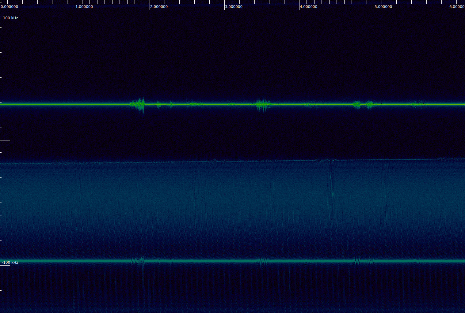
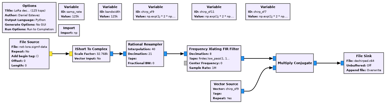
We can perform the first approach (dechirping at 125 ksps) with the following GNU Radio flowgraph. For simplicity I’m first using a rational resampler to convert the recording from 525 ksps to 1 Msps, and then use a Frequency Xlating FIR filter to downconvert and decimate the chirped signal of interest to 125 ksps. The two-sided bandwidth of the FIR filter is 140 kHz.
In the waterfall of the output we can see that the signal is now at a single frequency. We haven’t had to adjust the phase of the local chirp to align it with the received signal. The second FM signal that is visible in the waterfall corresponds to another flag, given by the weaker chirped signal that had the same parameters as flag 2 but a different chirp phase (note that its audio modulation is different).
However, the FM audio doesn’t sound so good, despite the fact that there are no frequency jumps. The result is somewhat worse than when we took care to adjust the phase of the local chirp by hand to match the received signal.
Let us think about why this happens. If we use an ideal chirp at continuous time and infinite bandwidth, it is true that the frequency difference between that chirp and a delayed version of the same chirp is always one of two frequencies spaced by 125 kHz. Moreover, as we will see in the appendix, the phase of the chirp is continuous. So the result of dechirping with an out-of-phase chirp is a signal that is phase continuous and jumps between two frequencies spaced by 125 kHz. If we are able to alias these two frequencies to the same one by sampling at 125 ksps, then it’s reasonable to think that we should get a phase-continuous signal at constant frequency, that is, a pure CW carrier. The key point here is that the chirp retraces instantly to the lower edge of its bandwidth when it reaches its upper edge.
If we consider either band-limited signals or discrete time (and considering discrete time implicitly brings all considerations about band-limited signals), this is no longer true. A band-limited signal cannot jump instantly in frequency. The band-limited version of the chirp takes some non-zero amount of time to retrace from the upper edge of the bandwidth to the lower edge. Likewise, in discrete time, the frequency between the two samples where the retrace happens will be a smudge of the upper edge and lower edge frequencies, rather than an instant frequency jump. Therefore, dechirping with an out-of-phase chirp in discrete time at 125 ksps introduces frequency glitches in the samples where the retrace of either the received signal or the local chirp happens. This is what deteriorates the quality of the FM audio.
I think that the reason why the audio quality with this trick is worse than if we don’t work at 125 ksps and try to match the chirp phase by hand is because when matching the chirp phase by hand we are also aligning the non-zero-time retraces of the received chirp and local chirp, so the retraces cancel out when multiplying by the complex conjugate. Even if we don’t align them within one sample, what we get is the effects of the two retraces close together in time (at a few samples distance) and with opposite sign. This probably cancels out somewhat in the audio lowpass filtering, and is less noticeable than when we work at 125 ksps, where we get the two retraces with opposite signs at completely different points of the chirp period.
I should say that there are more nuances regarding this discrete-time chirp retrace thing, and that arguably I made a small mistake when generating the chirps for the challenge. Since these details require some calculations, I have placed them in an appendix at the end of the post.
With all of these considerations we can get flag 2. I have already mentioned that flag 4 can be obtained with an AM receiver before dechirping. It can also be obtained by dechirping with the LoRa SF11 parameters, especially because AM is not so sensitive to chirp misalignment as FM.
Flag 3 is the weaker SF9 chirp that occupies the same bandwidth as flag 2 but is out of phase with it. A good way to get this flag is by manually adjusting the local chirp delay in the first GNU Radio flowgraph I’ve shown. Something around 1600 samples works well. The waterfall of the dechirped signal looks like this. The signal for flag 3 is the FM signal close to 0 Hz. Note that the copy of the signal 125 kHz away is not visible because the local chirp phase is adjusted relatively well.
Also note that the signal drifts up in frequency. I’ve put different sampling frequency offsets in all the signals (of reasonably realistic magnitudes around 1 to 10 ppm). This causes the alignment of the received chirp and the local chirp to change over time, and hence a frequency drift in the received signal. In flag 3 I threw in a larger sampling frequency offset of around 21 ppm. We could try to match the sampling frequency offset with our local chirp to cancel out the frequency drift, but it is easier to chase the frequency of the dechirped FM signal manually in GQRX.
The resulting audio is not great, but the flag can be copied with some effort.
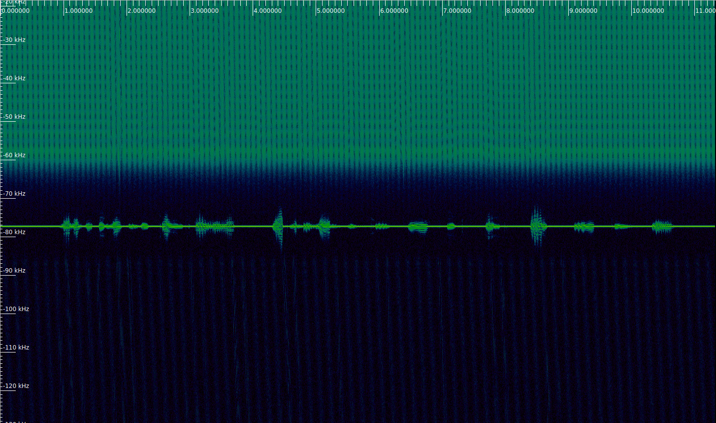
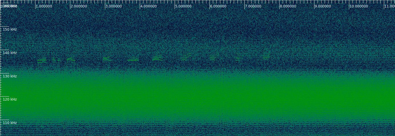
The remaining flag is flag 5. This is intended to be more difficult, so it is hiding almost below the noise floor. For this flag I used voice SSB modulation, so the power of the signal is proportional to my voice power and the signal can only be seen at the times where I raise my voice. I also used the chirp parameters from SF7. This is a faster chirp, which makes it more difficult to see the signal in the spectrum without dechirping. The signal is placed in the seemingly empty part of the spectrum of the SigMF recording. The fact that this part of the spectrum looks empty is intended to draw suspicion towards this area, especially for a participant that is only missing flag 5.
With significant effort it is possible to find some part of the recording and waterfall parameters which makes the chirps of the flag 5 signal slightly visible. Try to spot them in this figure. It is even possible to measure them and realize that they have the SF7 chirp rate.

Another approach is to blindly try different LoRa spreading factors and see if something shows up in the dechirped signal. Regardless of the approach, the outcome is to perform SF7 dechirping. This can be done with the same kind of GNU Radio flowgraph. Even without adjusting the delay of the local chirp, we can already see the SSB signal in the spectrum of the dechirped recording. There is some amount of interference from the other stronger signals, so results can be improved by filtering these out before dechirping, but this is not even necessary.
SSB is probably the most tolerant to local chirp misalignment of the three modulations I have used. In this case the flag can even be copied with the local chirp quite out of phase, but it pays off to play with the local chirp phase to improve the results and make the flag easier to copy. I have used a delay of 200 samples in the above GNU Radio flowgraph.
The dechirped SSB signal drifts slightly up in frequency, due to the sampling frequency offset. We can chase it by hand in GQRX, or leave the frequency somewhere were all the flag can be understood, despite being obviously mistuned, as I have done here.
Appendix
In this appendix I explain some of the subtleties of LoRa chirps in discrete time. The spreading factor will be denoted by \(S\), the bandwidth by \(B\), the chirp duration by \(T = 2^S/B\), and the sample rate by \(f_s\).
Consider the polynomial\[p(t) = \pi\left[\frac{B^2}{2^S}t^2 – Bt\right].\]A simple calculation shows that\[p(T/2 + t) = p(T/2 – t).\]In particular, \(p(T) = p(0)\). This means that the function \(\varphi\) defined as \(\varphi(t) = p(t)\) for \(0\leq t \leq T\) can be extended as a \(T\)-periodic continuous function to all \(\mathbb{R}\), which we also denote as \(\varphi\). This function gives the phase of the LoRa chirp waveform in continuous time, \(x(t) = e^{i\varphi(t)},\) because its instantaneous frequency in Hz is\[\frac{\varphi'(t)}{2\pi} = \frac{B^2}{2^S}t – \frac{B}{2},\qquad 0 < t < T,\]which is a linear slope between \(-B/2\) and \(B/2\) as required.
Let us consider the frequency difference between \(\varphi(t + \Delta)\) and \(\varphi(t)\). Without loss of generality we assume \(0 < \Delta < T\). Then\[\frac{\varphi'(t+\Delta)-\varphi'(t)}{2\pi} = \begin{cases}\frac{B^2\Delta}{2^S} & 0 < t < T – \Delta\\ \frac{B^2\Delta}{2^S} – B & T – \Delta < t < T\end{cases}.\]Therefore, excepts at the points \(t = kT\) and \(t = kT – \Delta\), for \(k \in \mathbb{Z}\), where \(\psi(t) = \varphi(t+\Delta) – \varphi(t)\) is not differentiable, the function \(\psi(t)\) has either one of two instantaneous frequencies, which differ by \(B\).
Now we consider the discrete time case. We assume that \(f_s\) is an integer multiple of \(B\), so that the chirp period is an integer number of samples \(N = 2^S f_s / B\). The most natural choice for a discrete time version of the LoRa chirp is \(e^{ia[n]}\), where\[a[n] = \varphi\left(\frac{n}{f_s}\right),\quad n \in \mathbb{Z}.\]Note that \(a[n]\) is \(N\)-periodic. In discrete time it does not make sense to speak of the instantaneous frequency. It only makes sense to speak about the average frequency between two samples. In units of Hz, this is given by\[\frac{a[n+1]-a[n]}{2\pi}f_s.\]A simple calculation shows that\[\frac{a[n+1]-a[n]}{2\pi}f_s = \frac{\varphi’\left(\frac{n+1/2}{f_s}\right)}{2\pi}.\]Therefore, with this choice of a discrete-time chirp, the average frequency between two samples is equal to the frequency of the continuous-time chirp at the midpoint between the two samples. This happens because the frequency of the continuous-time chirp is linear, so its average on an interval coincides with its value at the midpoint of the interval. Note that this equality is true even for \(n = kN-1\), \(k \in \mathbb{Z}\), because the derivative of \(\varphi\) is linear in the interval \((kN-1)/f_s < t < kN/f_s\).
As a consequence of this relation between the average frequency of \(a[n]\) and the instantaneous frequency of \(\varphi(t)\), we have that the difference between \(a[n+M]\) and \(a[n]\) has an average frequency between samples that is always equal to one of two values that differ by \(B\). In particular, if \(f_s = B\), since frequencies in discrete-time only have sense modulo \(f_s\), this means that the average frequency between samples is constant. This implies that the product of one of these discrete time chirps by the complex conjugate of a delayed version of the same chirp is a signal of constant frequency, a CW carrier.
However, \(a[n]\) is not the only reasonable choice for a discrete-time version of the chirp. We could have sampled the continuous-time chirp \(\varphi(t)\) at another set of points spaced by \(1/f_s\). We consider\[b[n] = \varphi\left(\frac{n+\delta}{f_s}\right),\qquad n \in \mathbb{Z}\] for some fixed \(0 < \delta < 1\). This sequence is also \(N\)-periodic. Now we still have\[\frac{b[n+1]-b[n]}{2\pi}f_s = \frac{\varphi’\left(\frac{n+\delta+1/2}{f_s}\right)}{2\pi},\qquad n \neq kN – 1,\ k \in \mathbb{Z},\]but this equality is not true anymore for \(n = kN – 1\), \(k \in \mathbb{Z}\). The reason is that \(\varphi'(t)\) is not linear between \((kN+\delta-1)/f_s\) and \((kN+\delta)/f_s\), because it has a jump discontinuity at \(t = kN/f_s\).
The consequence is that the phase difference between \(b[n+M]\) and \(b[n]\) has an average frequency between samples that is equal to either one of two values that differ by \(B\) except when \(n = kN – 1\) or \(n = kN – M – 1\), for \(k \in \mathbb{Z}\). For these points the average frequency is generally another different value (it depends on \(\delta\)). Therefore, when \(f_s = B\), the product of one of these chirps by the complex conjugate of a delayed version of the same chirp is almost always a signal of constant frequency, but it has “frequency glitches” at some samples.
So we have seen that \(a[n]\) has this nice property that the product of a chirp by the complex conjugate of a delayed version of the same chirp is a pure CW carrier, but when we use \(b[n]\) instead, we have glitches. Even though we can generate a sequence like \(a[n]\) and use it for signal processing in the receiver, in most practical situations the received signal looks more like a version of \(b[n]\). This is because we do not control the alignment of the samples with the received chirp frequency jumps, and also because the RF signal is band-limited. The nice property of \(a[n]\) happens only when the continuous-time signal is infinite bandwidth and the frequency jumps happen exactly at the sampling points, rather than in between samples.
Now to the “small mistake” that I made when generating the signals in the challenge. I wasn’t thinking too carefully and I designed my chirp directly in discrete time. I defined it as \(e^{ic[n]}\), where\[c[n] = 2\pi \sum_{k=0}^n \left(\frac{B^2k}{2^Sf_s} – \frac{B}{2f_s}\right), \qquad n = 0, 1, \ldots, N-1,\]extended as an \(N\)-periodic sequence to all \(\mathbb{Z}\). The motivation for this definition is that\[\frac{c[n+1]-c[n]}{2\pi f_s} = \frac{B^2}{2^s f_s}(n + 1) – \frac{B}{2},\qquad n = 0, 1, \ldots, N – 2.\]This is the linear slope we want. However, what is slightly awkward is that this difference quotient gives the average frequency between the samples \(n\) and \(n+1\), but however its value matches the instantaneous frequency that we should have at time \((n+1)/f_s\). Therefore, technically speaking this chirp is shifted in time by half a sample.
Indeed, a straightforward calculation shows that\[c[n] – \varphi\left(\frac{n + 1/2}{f_s}\right)\]is just a constant. This constant acts as a carrier phase offset in the chirp, so we can mostly ignore it. Therefore, the discrete-time chirps that I generated in the challenge looked like the sequence \(b[n]\) with \(\delta = 1/2\). In particular, the average frequency between the samples \(kN – 1\) and \(kN\) for \(k \in \mathbb{Z}\) is zero. This means that in this discrete time chirp the average frequency between samples grows as a linear slope, roughly from \(-B/2\) to \(B/2\), and then it passes through zero before returning again to the beginning of the linear slope. If this kind of sequence is used as local chirp instead of \(a[n]\) for the dechirping at \(f_s = B\) trick, it makes the frequency glitches quite evident. However, even if I had used \(a[n]\) everywhere, there would still be frequency glitches. This is because the received chirps do not have its frequency jumps aligned with sampling instants either, as I passed the chirps by a Polyphase Arbitrary Resampler to simulate a sampling frequency offset, and then resampled the recording to 525 ksps, which doesn’t give an integer number of samples per chirp.
One comment