On 2020-09-04, China launched a “reusable experimental spacecraft” of which very little is publicly known. The most popular hypothesis is that this is a robotic spaceplane similar to the X-37B. The spacecraft spent two days in orbit and landed back at Earth, most likely near Lop Nur nuclear test site. Marco Langbroek has a nice post detailing all we know about the mission.
During the time it spent in orbit, the spacecraft released an object which has been catalogued as 2020-063G and is commonly known as “Object A”. On 2020-09-14, Dmitry Pashkov R4UAB detected an S-band signal coming from Object A at around 2280 MHz. This was verified later by Scott Tilley VE7TIL, who received a strong signal with lots of fading, suggesting that the object is tumbling. Marco also did some optical observations of the object.
Scott has sent me a recording of the S-band signal that he did on 2020-09-15 so that I can analyse it and we can learn more about this mysterious object. This post shows the results of my analysis.
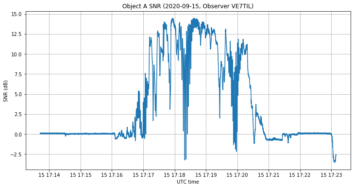
The figure below shows the SNR of the signal recorded by Scott. We see that the signal appears from the noise shortly after 17:16 UTC and quickly rises in strength up to almost 15dB of (S+N)/N. There are many deep fades, and after a couple of minutes the signal disappears in the noise again.
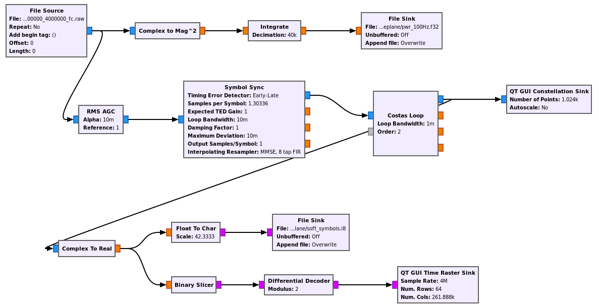
The modulation of the signal is BPSK at 3069kbaud. I have used this GNU Radio flowgraph to demodulate the signal. The flowgraph has nothing special. It is just a simple BPSK demodulator that saves soft symbols and average power measurements into files.
The analysis of the symbols is done in this Jupyter notebook. Before we begin looking at them, let me remark something interesting about the baudrate. The number 3069 equals 3 times 1023, and 1023 kHz is the basic chip rate of GNSS signals. The use of this number started with GPS, which uses 1023 chip Gold codes, so as to give a 1ms code repetition interval. Modern GNSS signals are all based on multiples of 1023 kHz chip rates even if they no longer use PRN lengths of 1023 chips.
Therefore, the choice of a 3069 kbaud baurate might suggest that this is some kind of ranging signal, using a ranging code of length 1023 that is perhaps based on a 10 bit LFSR. However, this doesn’t seem to be the case.
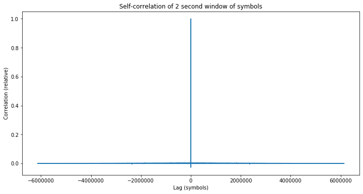
The signal is clearly differentially encoded. The figure below shows the self correlation of a 2 second window of the symbol stream chosen where the SNR is strongest, so as to have few bit errors. There is almost no self-correlation.
However, if we perform differential decoding on the symbol stream, we see a strong self-correlation at lags multiples of 261888 symbols. This suggests a frame size of 261888.
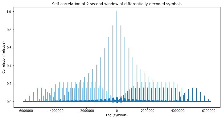
Note that 261888 equals 256 times 1023, so again we have the number 1023 showing up. From here on, we will work with the differentially-decoded bitstream. If we arrange the bitstream in rows of 261888 bits, we get the figure below, which has been produced with 60 seconds worth of symbols.
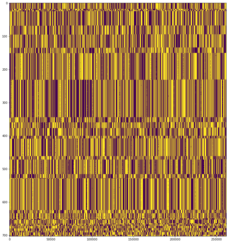
We see that all the frames consist of almost the same pattern of 261888 bits. Occasionally there is a deep fade and clock recovery is lost, so we jump to another phase of the cyclic pattern.
Upon a closer look, we see that there are some bits that change. For instance, the figure below shows the first 256 bits of each 261888 bit frame, in a segment of data where there are no jumps due to clock recovery failure. We see that there are 6 bits that toggle occasionally. All the other bits maintain a constant value.
Moreover, it seems that there is a regular spacing between the bit positions that toggle. It is not difficult to identify the list of bit positions that toggle sometimes. I have studied this list to try to understand what is happening here.
In particular, I was trying to find a reasonable deinterleaving scheme that placed all the bits that toggle at the beginning of the frame. My idea was that maybe were are looking at frames that are scrambled and interleaved, and only the beginning of the frames contains valid data, while the rest is zeros. Thus, we would be looking mostly at the interleaved scrambler pattern, and some bits that correspond to valid data and are separated by the interleaver stride. However, the pattern doesn’t seem so simple, and I haven’t been able to come up with a good explanation.
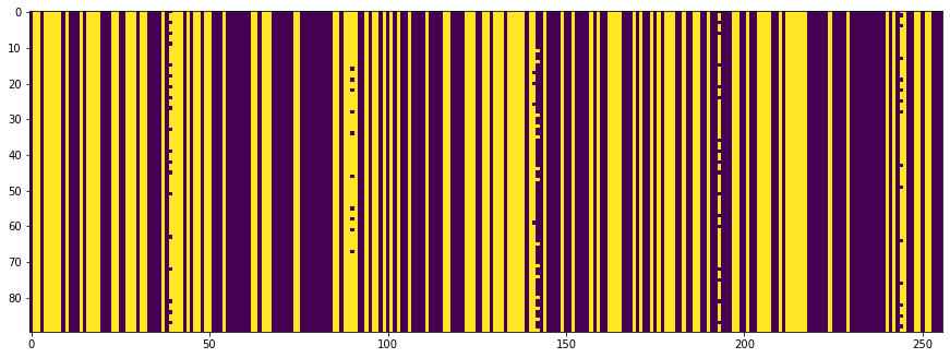
In any case, it is true that the bit positions that toggle are separated by a rather regular spacing. To show this, we proceed as follows. We colour in yellow those positions that can toggle, and in purple the positions that never toggle, so we come up with a list of 261888 positions that are either yellow or purple. Next, we arrange that list in rows of 51 elements. The figure below shows the first 50 of those rows. The pattern continues “snaking” towards the right (and looping back to zero) on the following rows.

We see that there are a few rows where a single yellow square appears in the same position. Then a new yellow square appears in the following position, and this state with two yellow squares per row persists for only one or two rows. In the next row the left yellow square disappears, so the pattern has moved one position to the right.
Alternatively, we can write our list of positions as a set of indices and show the quotient and remainder of these indices when divided by 51. Note that this is essentially the same as the figure above. The beginning of this list of quotient and remainder pairs looks like this (the line jumps have been added for clarity):
(0, 39),   (1, 39),  (2, 39),
(2, 40),   (3, 40),  (4, 40),  (5, 40),  (6, 40),  (7, 40),  (8, 40),  (9, 40),
(9, 41),  (10, 41), (11, 41), (12, 41), (13, 41), (14, 41), (15, 41),
(15, 42), (16, 42), (17, 42), (18, 42), (19, 42), (20, 42), (21, 42), (22, 42),
(22, 43), (23, 43), (24, 43), (25, 43), (26, 43), (27, 43), (28, 43),
(28, 44), (29, 43),
(29, 44), (30, 44), (31, 44), (32, 44), (33, 44), (34, 44), (35, 44),
(35, 45), (36, 44),
(36, 45), (37, 45), (38, 45), (39, 45), (40, 45), (41, 45), (42, 45),
(42, 46), (43, 46), (44, 46), (45, 46), (46, 46), (47, 46), (48, 46),
(48, 47), (49, 46),
(49, 47), (50, 47), (51, 47), (52, 47), (53, 47), (54, 47), (55, 47),
(55, 48), (56, 48), (57, 48), (58, 48), (59, 48), (60, 48), (61, 48), (62, 48),
(62, 49), (63, 49), (64, 49), (65, 49), (66, 49), (67, 49), (68, 49), (69, 49),
(69, 50), (70, 50), (71, 50), (72, 50), (73, 50), (74, 50), (75, 50),
(76, 0),   (77, 0),  (78, 0),  (79, 0),  (80, 0),  (81, 0),  (82, 0),  (83, 0),
(83, 1),   (84, 1), ....
I have no clue what we’re looking at here. The pattern shown in the figure above can be described by saying that it’s a series of vertical “sticks” that move to the right and overlap at their endpoints. However, the heights of these sticks vary. There are sticks of lengths 7, 8 and 9. The overlap also changes between one and two rows. So there is certainly a lot of regularity, but it isn’t a totally trivial pattern, such as the one produced by a matrix interleaver. It may happen that we’re missing to identify some bits that may toggle between different frames, but don’t.
I think that the fact that we have these toggling bits discards all ideas about a ranging code or a CDMA system. It wouldn’t make sense to toggle a few individual chips in such a system. It would also be quite strange to use differential encoding with a ranging code or CDMA signal.
An important remark is that these bits that toggle are not caused by symbol errors. Since we are doing differential decoding, a symbol error would cause two adjacent bits to toggle, which doesn’t happen here.
One thing is clear: the signal doesn’t have much data in it, as most of the bits show the same repeating pattern.
Here I end my analysis, since by now I don’t have any clever ideas to explain the structure we see in the bitstream. The original IQ file and the stream of soft symbols are too large to share conveniently, but in the Github repository I have included a file with the 60 seconds worth of differentially decoded symbols. This file has a size of only 22MB and it should be sufficient for anyone that wants to continue the analysis where I left it. The file can be downloaded with git-annex as indicated in the README.
Very interesting!