A couple years ago I wrote a post about the paper Controlled-Root Formulation for Digital Phase-Locked Loops, by Stephens and Thomas. In this paper, the authors study digital PLLs by studying the transfer function in discrete time, rather than doing any continuous-time approximations or equivalences. They give values for the loop coefficients that are needed to achieve a certain noise bandwidth for some standard loop root placements (the supercritical damped response and the standard underdamped response). In general, the loop coefficients are obtained numerically. In my post, I show that in the case of a loop of order 2 with supercritical response the loop coefficients can be calculated explicitly in terms of the loop bandwidth by using the solution of a cubic equation. However, in that post, I treated only the phase/phase-rate feedback case. In this post I cover the rate-only feedback case.
Throughout this post I will be using the same notation as in the Stephens and Thomas paper. The difference between the phase/phase-rate feedback and rate-only feedback cases is as follows. In a phase/phase-rate feedback system, the loop update computes the next model phase as \(\hat{\phi}_{n+1} = \hat{\phi}_n + \hat{\dot \phi}_{n+1} T\). The model phases \(\hat{\phi}_n\) are referred to the midpoint of the loop update interval, because the residual phase \(\tilde{\phi}_n\) obtained in that interval corresponds to the average residual phase over that interval (assuming that the input signal amplitude is constant), and hence is equal to the instantaneous residual phase at the midpoint of the loop update interval if we assume that the input signal phase is a linear function over the loop update interval. Therefore, to achieve an instantaneous phase of \(\hat{\phi}_{n+1}\) at the midpoint of the next interval, the local oscillator phase needs to be reset to a value of \(\hat{\phi}_{n+1} – \hat{\dot \phi}_{n+1} T / 2 = \hat{\phi}_n + \hat{\dot \phi}_{n+1} T / 2\) at the beginning of the next interval. This value is different in general from the value that the local oscillator phase has at the end of the current interval, which is \(\hat{\phi}_n + \hat{\dot \phi}_n T / 2\). Therefore, phase/phase-rate feedback requires phase jumps in the local oscillator. If the system has a phase-continuous local oscillator, then the local oscillator phase at the midpoint of the next interval will be \(\hat{\phi}_{n+1} = \hat{\phi}_n + (\hat{\dot \phi}_{n+1} T + \hat{\dot \phi}_n T)/2\). This case is the rate-only feedback system.
Generally speaking, phase/phase-rate loops are better because the rate-only system introduces a certain delay in the loop update, which make the loop behave worse, specially for large \(B_L T\). However, in some cases having continuous local oscillator phase is a system design requirement. Note that the phase/phase-rate versus rate-only distinction applies only when the loop integrates multiple samples to produce a phase estimate before running the loop update. When the loop update is performed every sample, the two cases collapse into one case that has the same transfer function as the phase/phase-rate case but also has continuous phase.
The paper by Stephen and Thomas shows that in the phase/phase-rate case, the loop transfer function of an order \(N\) loop is\[H_z(z) = \frac{D(z) – (z-1)^N}{D(z)},\]where\[D(z) = (z-1)^N + (z-1)^{N-1}K_1 + z(z-1)^2 K_2 + \cdots z^{N-1}K_N.\]They mention that the transfer function for the rate-only case can be calculated analogously, but they do not show the result. Carrying out these calculations we can see that it is\[H_z(z) = \frac{D(z) – z(z-1)^N}{D(z)},\]where\[D(z) = z(z-1)^N + \frac{1}{2}(z+1)[(z-1)^{N-1}K_1 + z(z-1)^2 K_2 + \cdots z^{N-1}K_N].\]The first thing we notice in contrast with the phase/phase-rate feedback case is that in the rate-only feedback case \(D(z)\) has degree \(N + 1\) instead of \(N\). This means that there is one additional loop root, which is caused by the update delay.
In Table IV, the paper gives formulas for the normalized loop bandwidth \(B_L T\) in terms of the loop coefficients \(K_1, \ldots, K_N\) for \(N = 1, 2, 3, 4\) for the phase/phase-rate feedback case. An equivalent table for the rate-only feedback case is not given. To compute the loop bandwidth for the rate-only feedback case we proceed as in the paper. The paper shows that\[2 B_L T = \frac{1}{2 \pi i}\oint H_z(z) H_z(z^{-1}) z^{-1}\, dz,\]where the contour integral is along the unit circle. It mentions that all the poles of \(H_z(z)\) need to lie inside the unit disk for the loop to be stable, and so the only poles of the integrand are the loop roots \(z_j\), which are the roots of the polynomial \(D(z)\), which all need to be inside the unit disk. Therefore, when all these roots are simple, the integral can be evaluated as\[2 B_L T = \sum_{j} [(z – z_j) H_z(z)H_z(z^{-1})z^{-1}]_{z\to z_j}.\]
The paper does not comment this, but it is clear that it is enough to study the case when all the roots are simple, because it is the generic case. This is because \(B_L T\) depends continuously on the loop coefficients and by applying a small perturbation to the loop coefficients we can make all roots simple. Writing\[D(z) = (z – z_0) \cdots (z – z_N),\]the expression above becomes\[2 B_L T = \sum_{j = 0}^N (D(z_j) – z_j(z_j – 1)^N) H(z_j^{-1}) z_j^{-1} \prod_{k \neq j} \frac{1}{z_j – z_k}.\]
Observe that the expression on the right hand size is a rational function with variables \(z_0, \ldots, z_N, K_1, \ldots, K_N\) that is symmetric in \(z_0, \ldots, z_N\). Therefore, it can be rewritten as a coefficient of polynomials in the elementary symmetric polynomials\[\begin{split}e_1(z_0, \ldots, z_N) &= z_0 + \cdots + z_N,\\e_2(z_0, \ldots, z_N) &= z_0z_1 + z_0z_2 + \cdots + z_{N-1}z_N,\\ e_{N+1}(z_0, \ldots, z_N) &= z_0z_1\cdots z_N\end{split}\]with coefficients on \(\mathbb{Q}[K_1, \ldots, K_N]\). Since\[\begin{split}D(z) = &z^{N+1} – e_1(z_0, \ldots, z_N) z^{N-1} + e_2(z_0, \ldots, z_N) z^{N-2} + \cdots + \\ &+ (-1)^{N+1} e_{N+1}(z_0, \ldots, z_N),\end{split}\]we can obtain expressions for these elementary symmetric polynomials in terms of \(K_1, \ldots, K_N\) by expanding the definition of \(D(z)\). Replacing these expressions into the above, we obtain an expression for \(2 B_L T\) that is a rational function in \(K_1, \ldots, K_N\).
These calculations are very cumbersome to carry out by hand if \(N \geq 2\), but they can easily be performed with a computer algebra system. The only things that are required are multivariate rational function algebra, and rewriting a symmetric polynomial in terms of elementary symmetric polynomials. I have written some code using SageMath that performs these calculations for both the phase/phase-rate and the rate-only cases. For the phase/phase-rate case I can replicate the results of Table IV in the paper, although I have not checked carefully that the expressions I obtain for \(N = 3, 4\) are the same, since they are pretty large.
Note that for \(N = 1\) it turns out that the loop bandwidth is\[B_L T = \frac{K_1}{4 – 2 K_1}\]for both phase/phase-rate feedback and for rate-only feedback, even though the loop transfer function is different. This means that the same loop coefficient choice serves for both cases.
The next thing we are interested in is computing the loop coefficients \(K_1, K_2\) for \(N = 2\) for supercritical damping in the rate-only feedback case, given a fixed loop bandwidth \(B_L T\). Generally speaking, supercritical damping means that all the loop roots are equal to some real number \(e^{-\beta}\), \(\beta > 0\). However, in the rate-only feedback case there is one additional loop root due to the update delay. Therefore, only \(N\) loop roots can be equal. The remaining root is determined by the rest. For \(N = 2\) we set \(z_1 = z_2 = w = e^{-\beta}\), and \(z_0 = v\).
Writing the coefficients of \(D(z)\) in terms of the elementary symmetric polynomials in the loop roots, we obtain the following equations:\[\begin{split}w^2 v &= \frac{1}{2}K_1, \\ w^2 + 2wv &= \frac{1}{2}K_2 + 1, \\ 2w + v &= 2 – \frac{1}{2}K_1 – \frac{1}{2} K_2.\end{split}\]The first two of these equations give expressions for \(K_1\) and \(K_2\) in terms of \(w\) and \(v\). Replacing \(K_1\) and \(K_2\) by these expressions in the last equation, we obtain that\[v = \frac{- w^2 – 2w + 3}{w^2 + 2w + 1}.\]Substituting in the first two equations, we get\[\begin{split}K_1 &= \frac{-2w^4 – 4w^3 + 6w^2}{w^2 + 2w + 1},\\K_2 &= \frac{2w^4 – 8w^2 + 8w – 2}{w^2 + 2w + 1}.\end{split}\]
The loop bandwidth is\[B_L T = \frac{2K_1^2 + K_1K_2 + 2K_2}{-4K_1^2 – 2K_1K_2 + 8K_1 – 4K_2}.\]Replacing the above expressions in this formula, we get\[B_L T = \frac{-w^6 – 6w^5 – 5w^4 + 12 w^3 – w^2 + 2w – 1}{2w^6 + 12w^5 – 14w^4 – 8w^3 + 14w^2 – 4w + 2}.\]This gives a degree 6 equation for \(w\) in terms of \(B_L T\). Unfortunately, degree 6 equations do not have a closed form solution in general. In the phase/phase-rate case that I treated in the older post, we obtained a degree 3 equation, so we could obtain an explicit formula for its solution involving some cubic roots. In this case, all we can do is to solve this equation numerically. We compute the roots of the resulting degree 6 polynomial, and choose as \(w\) the largest real root in the interval \((0, 1)\). It is easy to see that if \(B_L T \to 0\), then \(w \to 1\). Therefore, it is quite likely that a good way to solve this problem numerically is to begin with \(w = 1\) and apply an iterative algorithm such as Newton’s method. Once we have obtained a solution \(w\), we can compute \(K_1\) and \(K_2\) by using the formulas above.
The rational function that gives \(B_L T\) in terms of \(w\) has a maximum value of 0.22137 when \(0 < w < 1\). This gives the maximum loop bandwidth that can be realized with this loop. Compare with the phase/phase-rate feedback case, which supports a maximum loop bandwidth of \(B_L T = 3/2\).
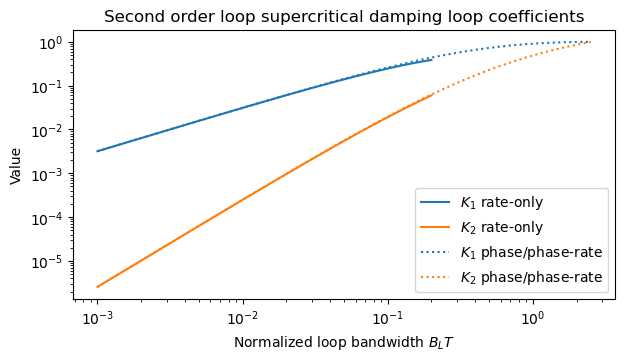
The following post compares the loop coefficients \(K_1\), \(K_2\) that are obtained for different choices of \(B_L T\) for the phase/phase-rate feedback case (for which explicit formulas were obtained in the older post) and for the rate-only feedback case. We see that both cases give very similar coefficients when the loop bandwidth is small. This makes intuitive sense, because the update delay of the rate-only feedback case has a smaller effect when the loop bandwidth is smaller.
The next figure shows the relative difference between the coefficients of the two cases.
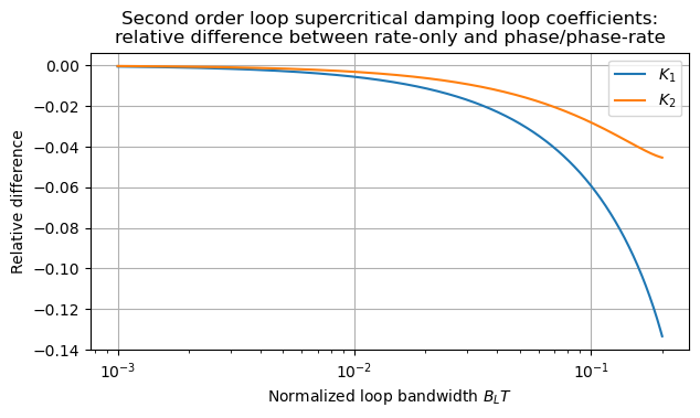
This figure suggest that since the rate-only feedback case does not have an explicit formula for the loop coefficients, we can design the coefficients for the phase/phase-rate case and simply apply them to the rate-only case. However, there is a better way, since the issue with this approach is that we break all the loop properties, including the supercritical damping.
The challenge in the rate-only feedback case is that we get an equation of degree 6 for \(B_L T\) in terms of \(w\). A key idea is that in most applications we do not need to solve this equation exactly. We can obtain an approximation for \(w\), which has the effect of making a small error in the loop bandwidth. Then we can still compute \(K_1\) and \(K_2\) in terms of \(w\), obtaining a loop that has supercritical damping, with the only caveat that the loop bandwidth is slightly different from the design target.
To this end, we can compute the Padé approximant of degree 2 of the rational function for \(B_L T\) in terms of \(w\) at \(w = 1\), obtaining\[B_L T \approx -\frac{25(47 w^2 – 60 w + 13)}{16 (131 w^2 – 102 w + 56)}.\]This approximation tends to the exact value as \(B_L T \to 0\). Since this gives an equation of degree 2 for \(w\), we can solve it explicitly, obtaining\[w \approx \frac{816 B_L T + \sqrt{-1212160 (B_L T)^2 – 510000 B_L T + 180625} + 750}{2096 B_L T + 1175}.\]Replacing this approximation for \(w\) in the formulas above for \(K_1\) and \(K_2\), we obtain explicit formulas for the loop coefficients that give supercritical damping exactly and a loop bandwidth that is approximately \(B_L T\).
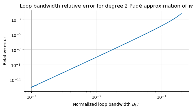
The following figure shows the relative error in \(B_L T\) that we get by using this approximation. We can see that it is quite small. In most applications an error of 1% or less in the loop bandwidth makes absolutely no practical difference.
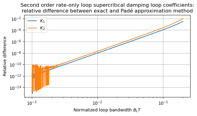
The next plot shows the relative difference between the loop coefficients \(K_1\) and \(K_2\) obtained with this Padé approximation method and the exact loop coefficients.
It is also possible to use a Padé approximant of degree 3, in which case we obtain a cubic equation that can also be solved explicitly. However, the expressions that are obtained are very complicated, so this is not worth the effort.
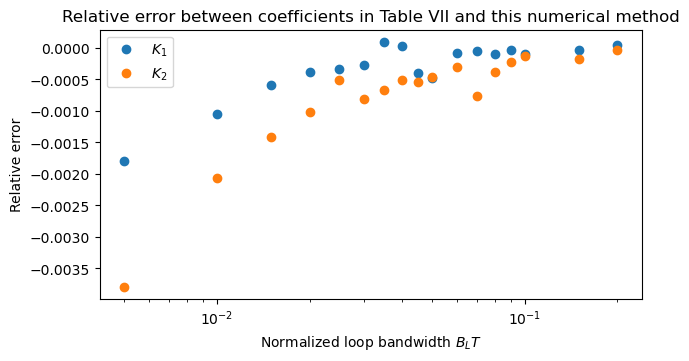
Table VII in the paper contains loop coefficients for the rate-only feedback case with supercritical damping for some choices of \(B_L T\). In the plot below we show the relative error between the coefficients in this table and coefficients calculated by solving exactly the value of \(w\) in terms of \(B_L T\) by using numerical root finding. We see that there is a bias in the coefficients in the paper that grows as \(B_L T \to 0\). The reason for this is unknown. Perhaps there was a small error in the numerical method used to obtain the results in the paper. Something I noticed is that the paper shows slightly different \(K_1\) values for \(N = 1\) in the phase/phase-rate and rate-only feedback cases, while \(K_1\) should be exactly the same in both cases, since the formula for \(B_L T\) in terms of \(K_1\) is the same.
The calculations done for this post are in this Jupyter notebook.