I have published a new Python package called sigmf-toolkit. It is intended to be a collection of Python tools to work with SigMF files. At the moment it only contains two tools, but I plan on adding more tools to this package as the needs arise. These tools are:
gr_meta_to_sigmf. It converts a GNU Radio metadata file with detached headers to a SigMF file. At the moment it is really simple, and it doesn’t handle capture discontinuities.- sigmf_pcap_annotate. This tool parses a PCAP file using Scapy and it adds annotations to a SigMF file for each packet in the PCAP file.
I find this sigmf_pcap_annotate tool quite useful when comparing side by side a SigMF file in Inspectrum and a PCAP file in Wireshark to debug issues with digital communications systems. In this post I showcase how this tool can be used.
As an example communications system I have decided to use one of the examples from my gr4-packet-modem project. The reason is that this project is a packet-based modem with IP communications and constant data rate, and there are examples that can run without any hardware. Therefore, it is ideal for what I want to show.
I have basically followed the quick start guide of the project and configured Linux network namespaces by running the script scripts/netns-setup in the project checkout and then running the project’s pre-built Docker image as indicated:
docker run --rm --net host --user=0 \
    --cap-add=NET_ADMIN --cap-add=SYS_ADMIN \
    --device /dev/net/tun -v /var/run/netns:/var/run/netns \
    -it ghcr.io/daniestevez/gr4-packet-modem-built
The packet_transceiver example application contains the following data path: TUN device -> packet transmitter -> channel model -> packet receiver -> TUN device. The two TUN devices live in different network namespaces, and there is a veth linking the network namespaces so packets can flow in the opposite direction over virtual networking to allow two-way communications.
There is a small modification that needs to be done to the packet_transceiver application to write the output of the channel model to an IQ file. The following snippet of code needs to be added here.
auto& file_sink =
  fg.emplaceBlock<gr::packet_modem::FileSink<c64>>(
      {{"filename", "/tmp/iq.bin"}});
if (fg.connect<"out">(add_noise).to<"in">(file_sink) !=
    gr::ConnectionResult::SUCCESS) {
    throw gr::exception(connection_error);
}
After adding this snippet, the example can be rebuilt by running make in the build directory of the Docker container.
Now I run the following command to capture IP packets to a PCAP file in the gr4_tx network namespace, which corresponds to the transmit part of the example. This captures on any interfaces, so we will see both the packets in the TUN that goes to the transmitter, as well as replies flowing back through the veth.
sudo ip netns exec gr4_tx tcpdump -ni any -w gr4_tx.pcap
I also start a ping with the requests flowing through the modem and the replies flowing through the veth back channel.
sudo ip netns exec gr4_tx ping -i 0.01 192.168.10.2
Finally, the packet_transceiver example is run inside the Docker container as indicated in the quickstart guide.
/home/user/gr4-packet-modem/build/apps/packet_transceiver \
    20.0 0.005 1.2 0
After running the packet_transceiver for a couple of seconds, I stop it and copy the file /tmp/iq.bin out of the Docker container. I don’t have any timestamp associated with the start of this file, so I generate a timestamp with the following questionable method, which has enough accuracy for this simple demo.
I run stat on the Docker container to get the last timestamp of modification of the file, and wc -c to get the length of the file.
# stat /tmp/iq.bin
  File: /tmp/iq.bin
  Size: 38318080  	Blocks: 74840      IO Block: 4096   regular file
Device: 0,73	Inode: 141416      Links: 1
Access: (0644/-rw-r--r--)  Uid: (    0/    root)   Gid: (    0/    root)
Access: 2025-11-02 09:40:22.818611872 +0000
Modify: 2025-11-02 10:04:49.944612948 +0000
Change: 2025-11-02 10:04:49.944612948 +0000
 Birth: 2025-11-02 09:32:46.713488799 +0000
# wc -c /tmp/iq.bin
38318080 /tmp/iq.bin
Since the sample rate is 3.2 Msps and the file is complex64, so it has 8 bytes per sample, a timestamp corresponding to the beginning of the file can be calculated in Python as follows:
>>> np.datetime64('2025-11-02T10:04:49.944612948') \
  - np.timedelta64(round(38318080/(8 * 3.2e6) * 1e9), 'ns')
np.datetime64('2025-11-02T10:04:48.447812948')
I use this timestamp to write a simple .sigmf-meta file by hand, with the following contents.
{
    "global": {
        "core:datatype": "cf32_le",
        "core:num_channels": 1,
        "core:sample_rate": 3200000,
        "core:version": "1.2.5"
    },
    "captures": [
        {
            "core:datetime": "2025-11-02T10:04:48.447812948Z",
            "core:frequency": 400000000.0,
            "core:sample_start": 0
        }
    ],
    "annotations": [
    ]
}
To run the sigmf_pcap_annotate tool, I need to use the following parameters:
- Bits per second. The tool requires this parameter to convert the length of a packet in the PCAP to an over-the-air duration. This gr4-packet-modem example uses 800 ksym QPSK with no FEC, so the bit rate is 1.6 Mbps.
- Air overhead. Generally packets transmitted over the air have preambles that are not present in the decoded packet in the PCAP. The air overhead parameter is used to take this into account. In the case of the gr4-packet-modem example, there is a 64-bit BPSK syncword and a 128-bit QPSK physical layer header. The effective length of these two fields is 256 bits, since we have used 1.6 Mbps as the data rate.
The tool is run as follows:
sigmf_pcap_annotate \
    --pcap-file gr4_tx.pcap --sigmf-file iq.sigmf-meta \
    --bps 1.6e6 --air-overhead 256 --frequency 400e6 \
    --bandwidth 1e6
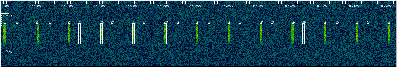
In Inspectrum we can see annotations corresponding to each of the packets in the PCAP file. The annotations start at the packet timestamp indicated in the PCAP file, and their duration is determined by the length of the packet in the PCAP file and the arguments given to the tool.
Generally speaking, annotations for a packet that is transmitted will begin at the point when the packet is created (in this case, when ping sends the packet into the TUN device). The burst corresponding to the packet in the IQ file might appear later if there is transmit latency or several packets queued up for transmission. For packets received over the air, the annotation will begin at the point when the packet is fully received by this system (in this case, when the packet arrives into the gr4_tx namespace veth). This means that these annotations appear strictly after the packet burst in the IQ file, since the receiver needs to see the whole burst to decode the packet. This quirk might be a feature rather than a bug depending on how we use it.
In this particular example the ping requests align pretty well with the transmit bursts, which means there is little transmit latency (or better said, the timestamp I have derived for the IQ data is not accurate enough to measure transmit latency). The ping replies flow over the veth, so they do not appear in the IQ file. Nevertheless, their annotations are quite useful. The time between the start of a ping request annotation and its corresponding ping reply annotation is around 3.2 ms. This is the round-trip-time that ping was reporting. The time between the end of a ping request annotation and the start of its corresponding ping reply annotation is around 2.6 ms. This time corresponds to receiver latency, assuming that the time for the packet to travel back over the veths is negligible.
The following shows the PCAP file in Wireshark. The numbers of the annotations in Inspectrum correspond to the packet numbers that are shown in Wireshark. This is crucial when trying to cross-reference interesting events in the SigMF and PCAP files.
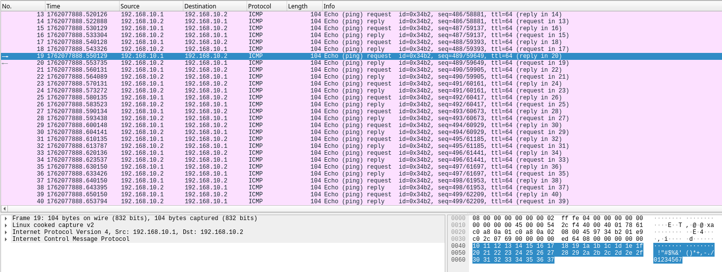
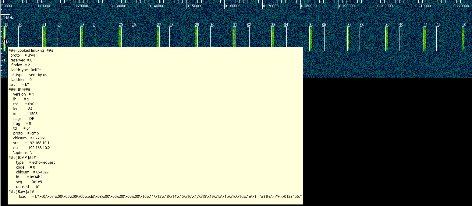
Since Scapy can parse the packets in the PCAP file and dump them in human-readable format, this dump is included in the comment field of each annotation. The comment can be shown in Inspectrum as a tooltip when hovering the mouse over an annotation. This is another useful way of quickly inspecting the upper layer data.
The example files that I have used in this post can be found in the dataset Example of SigMF file containing PCAP annotations in Zenodo.