Decoding the Artemis I Orion vehicle

On Wednesday 16th, the Artemis I mission was launched from Kennedy Space Center. This mission is the first (uncrewed) flight of the Orion Multi-Purpuse Crew Vehicle that will be used to return humans to the Moon in the next few years. Together with Orion, ten cubesats with missions to the Moon and beyond were also launched.

Seven hours after launch, I used two spare antennas from the Allen Telescope Array to record RF signals from Orion and some of the cubesats. By that time, the spacecraft were at a distance of 72000 km, increasing to 100000 km during the 3 hours that the observations lasted.

I have collected a lot of data on those observations, around 1.7 TB of IQ recordings. I am going to classify and reduce this data, with the goal of publishing it on Zenodo. Given the large amount of data, this will take some time. I will keep posting in this blog updates on this progress, as well as my results of the analysis of these signals.

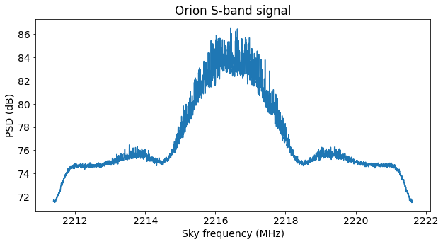
Today’s post is about Orion’s S-band main telemetry signal, which is transmitted at 2216.5 MHz. This signal has attracted great interest in the spacecraft tracking community because back in August NASA published an RFI giving the opportunity to ground stations belonging to private companies, research institutions, amateur associations and private individuals to track the S-band signal and provide Doppler data to NASA. Some of the usual contributors of the amateur space tracking community, including Dwingeloo’s CAMRAS (see their results webpage), Scott Chapman K4KDR and Scott Tilley VE7TIL (see his Github repository) are participating in this project.

Shortly after Artemis I launched, Amateur observers in Europe, such as Paul Marsh M0EYT, the Dwingeloo 25m radiotelescope, Ferruccio Andrea IW1DTU, Roland Proesch DF3LZ, were the first to receive the signals. They were then followed by those in America.

Summary

r00t.cz was the first to take a look to the signal modulation and coding, finding what I’m going to state in this section. The Orion telmetry signal at 2216.5 MHz is 2 Mbaud OQPSK. It uses CCSDS LDPC with r=1/2, k=1024. All the useful data seems to be encrypted.

There is a second type of modulation used by the same transmitter. This was noticed first by Roland, I think. It has a strong residual carrier. I haven’t looked at recordings of that modulation yet (and I didn’t manage to record it with the ATA), so that will be the topic for another post.

OQPSK demodulation

OQPSK is a very interesting modulation that occupies the realm between PAM modulations and continuous-phase frequency modulations. OQPSK is simply a QPSK modulation where the quadrature component has been delayed by half a symbol period, so that the symbol changes in the in-phase and quadrature components are staggered rather than simultaneous. With a half-sine pulse shape, OQPSK is constant-envelope, and is exactly the same as MSK, which is continuous-phase frequency shift keying with a deviation of 1/4th of the symbol rate and rectangular pulses (though there is a technical detail regarding differential coding; see Figure 2.4.17A-1 in the RF and Modulation Systems Blue Book).

Conversely, as shown by Laurent in the paper Exact and Approximate Construction of Digital Phase Modulations by Superposition of Amplitude Modulated Pulses (AMP), modulations related to MSK (including GMSK) can be written as PAM waveforms, perhaps with the addition of some terms that depend on “higher-order terms” of the symbol sequence. This remark can be used to treat MSK waveforms as if they were PAM, and demodulate them coherently.

However, when dealing with OQPSK the pulse shape is very important. For instance, depending on the pulse shape the waveform will be constant-envelope or not. I don’t know the exact pulse shape that Orion uses. I am interested in measuring it using the recordings that I’ve done, but I haven’t had the time yet.

I know that the pulse shape isn’t SRRC (square-root raised cosine), which is recommended by CCSDS for Category A spacecraft (see for instance footnote 5 in page 2.4.17A-1 in the Radio Frequency and Modulation Systems Part 1 Blue Book). Note that as in the case of BPSK and QPSK, the spectrum of an OQPSK modulation with a random symbol sequence is the Fourier transform of the time-domain pulse. In the ATA recording we can see that the modulation has sidelobes which are some 10 dB down from the main lobe. An SRRC pulse has no sidelobes.

The modulation isn’t constant envelope. The Fourier transform of the amplitude shows a strong component at 4 MHz, which is twice the baudrate. Therefore, the pulse is neither a half-sine pulse nor a perfect rectangular pulse. I suspect that the pulse shape is some kind of low-pass filtered rectangular pulse. The 3rd harmonic of a square wave is 9.54 dB below the fundamental, which roughly matches what we see in the spectrum. Therefore, the pulse filter probably lets the 3rd harmonic through with little attenuation but cuts off higher order harmonics.

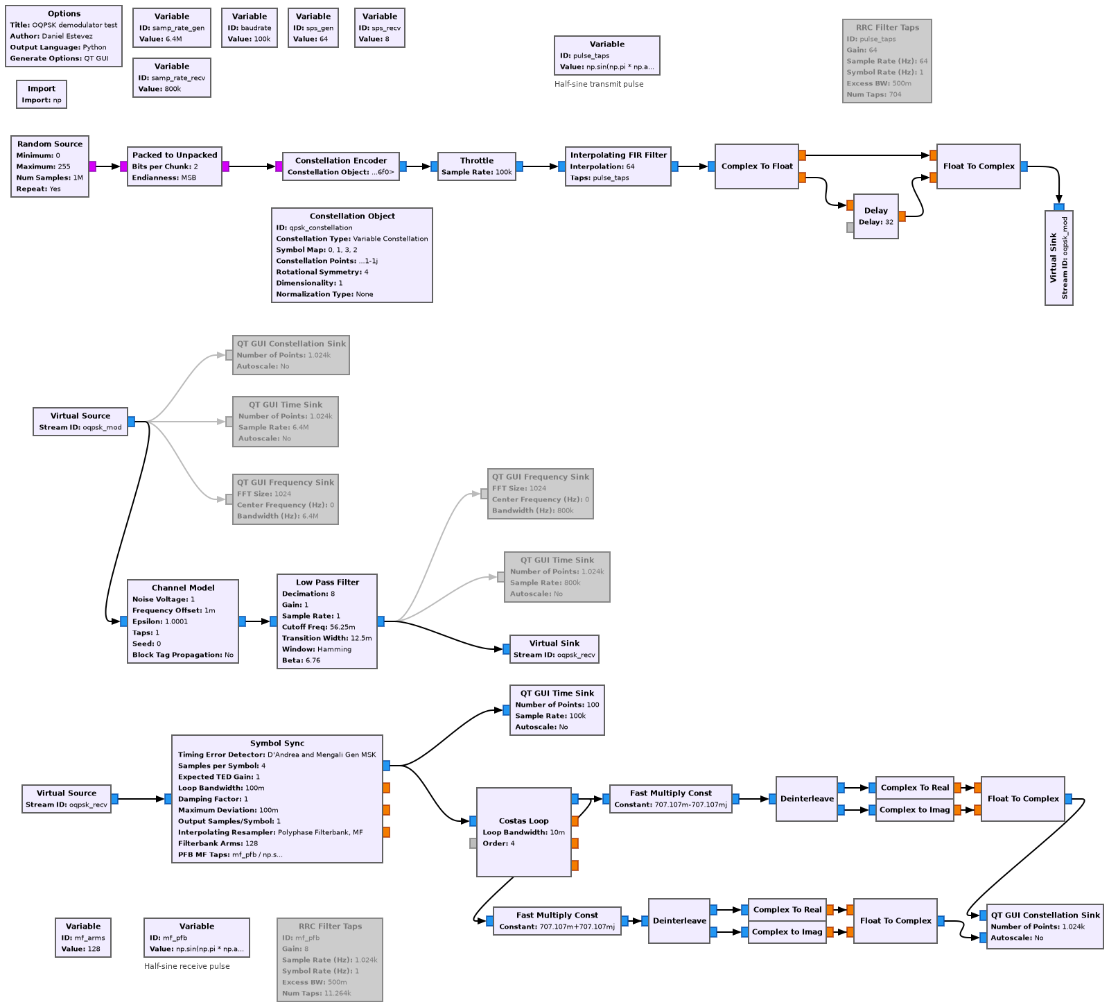
I was hoping to use a demodulator based on the generalized MSK time error detector proposed by D’Andrea, Mengali and Regianni, mainly because I participated in a discussion about its implementation in GNU Radio last year, but never had the chance to use it in a real world scenario. I prototyped a GNU Radio flowgraph that was working well for half-sine shaped OQPSK, but discovered that it doesn’t work at all for SRRC OQPSK nor for the Orion signal. The test flowgraph I have done using this method is called oqpsk_demodulator.grc and can be seen below.

More clues about the modulation of the signal can be obtained by computing the fourth power of the signal, \(x(t)^4\), where \(x(t)\) denotes the time-domain complex baseband signal. The Fourier transform of \(x(t)^4\) may show a CW tone at four times the carrier frequency. Whether this actually happens or not again depends on the pulse shape. For half-sine pulse OQPSK, there is no such component, because \(x(t)\) is uniformly distributed over the unit circle (and so the same happens with \(x(t)^4\)). On the other hand, for rectangular pulse OQPSK, \(x(t)^4\) will be a perfect complex exponential of constant frequency, so all the signal power will contribute to producing a CW tone in \(x(t)^4\). We see that the strength of this tone roughly depends on how fast the transitions between symbols happen.

The presence of this CW tone in \(x(t)^4\) means that we can lock a Costas loop before symbol synchronization and before undoing the staggering of the in-phase and quadrature branches. I originally got this idea from SatDump’s OQPSK demodulator. Depending on the pulse shape, it might happen that little signal power contributes to this CW tone. However, since this is a wideband signal at an appropriate Eb/N0 to decode it, and since we can use use a narrow bandwidth for the Costas loop because the signal dynamics change slowly, we see that the product of the signal C/N0 and the loop bandwidth is quite large. Therefore, the Costas loop will still have a high loop SNR even if only a small fraction of the signal power ends up contributing to producing this CW tone in \(x(t)^4\).

This trick of obtaining a CW tone in \(x(t)^4\) has been used by some of the Amateur observers to measure Doppler, since they do not have a working OQPSK demodulator. However, the trick doesn’t work in very low SNR conditions (when the Eb/N0 is way too weak for decoding the data), due to squaring losses. To measure the Doppler in low SNR, other techniques such as correlation against know parts of the signal (ASMs and/or idle frames) could be more useful.

At the Costas loop output we can delay the in-phase component to undo the staggering of the in-phase and quadrature-components. To simplify this delay, we have first resampled the signal to 4 samples per symbol, so that the delay is an integer number of samples (2 samples). At this point we obtain a regular QPSK modulation, so we can use the Symbol Sync block as usual. For simplicity I’m using a rectangular pulse shape filter on the receiver rather than a matched filter, since I don’t know the exact pulse shape used by the transmitter.

The Costas loop has a 90º degree ambiguity that needs to be handled. A moment’s thought shows that if the Costas has locked with a 180º error then we simply get the signals inverted at the output. However, consider what happens if the Costas has locked with an error of 90º, meaning that we’re getting the original signal plus an extra 90º rotation. In this case, the real part we see actually corresponds to minus the transmitted imaginary part, and the imaginary part we see corresponds to the transmitted real part. As we are delaying the received real part by half a symbol, the transmitted imaginary part has accumulated a total delay of one symbol, so it has been paired up with the wrong transmitted real symbol. To fix this, we need to delay the received imaginary symbols by one symbol, and also change the sign of the received real symbols. Then the real and imaginary parts need to be swapped.

If this sounds too confusing, maybe writing the same in equations is clearer. If \(T_I^n\) and \(T_Q^n\) are the transmitted real and imaginary parts for the symbol \(n\), at the output of the Costas loop we receive \(R_I^n = -T_Q^n\), \(R_Q^n = T_I^n\). However, when we form the symbols we apply a delay to the real part, so we end up with \(S_I^n = -T_Q^{n-1}\), \(S_Q^n = T_I^n\). To fix this, we form the output as \(O_I^n = S_Q^{n-1}\), and \(O_Q^n = -S_I^n\). By performing a substitution, we see that \(O_I^n = T_I^{n-1}\), \(O_Q^n = T_Q^{n-1}\), so we end up with the symbols in their correct branch and correctly paired up.

The case when the Costas loop has a phase error of 270º is like the 90º degree case except that we end up with inverted signals at the output. Therefore, the demodulator has two branches, one where nothing special is done, and another where the tricky thing described above is done. At the output of each branch, the CCSDS 64-bit ASM is searched both in the symbol stream and in the inverted symbol stream. In this way, the four possible cases of the Costas loop ambiguity are taken into account.

The GNU Radio demodulator flowgraph is shown below. The flowgraph is called orion_oqpsk.grc.

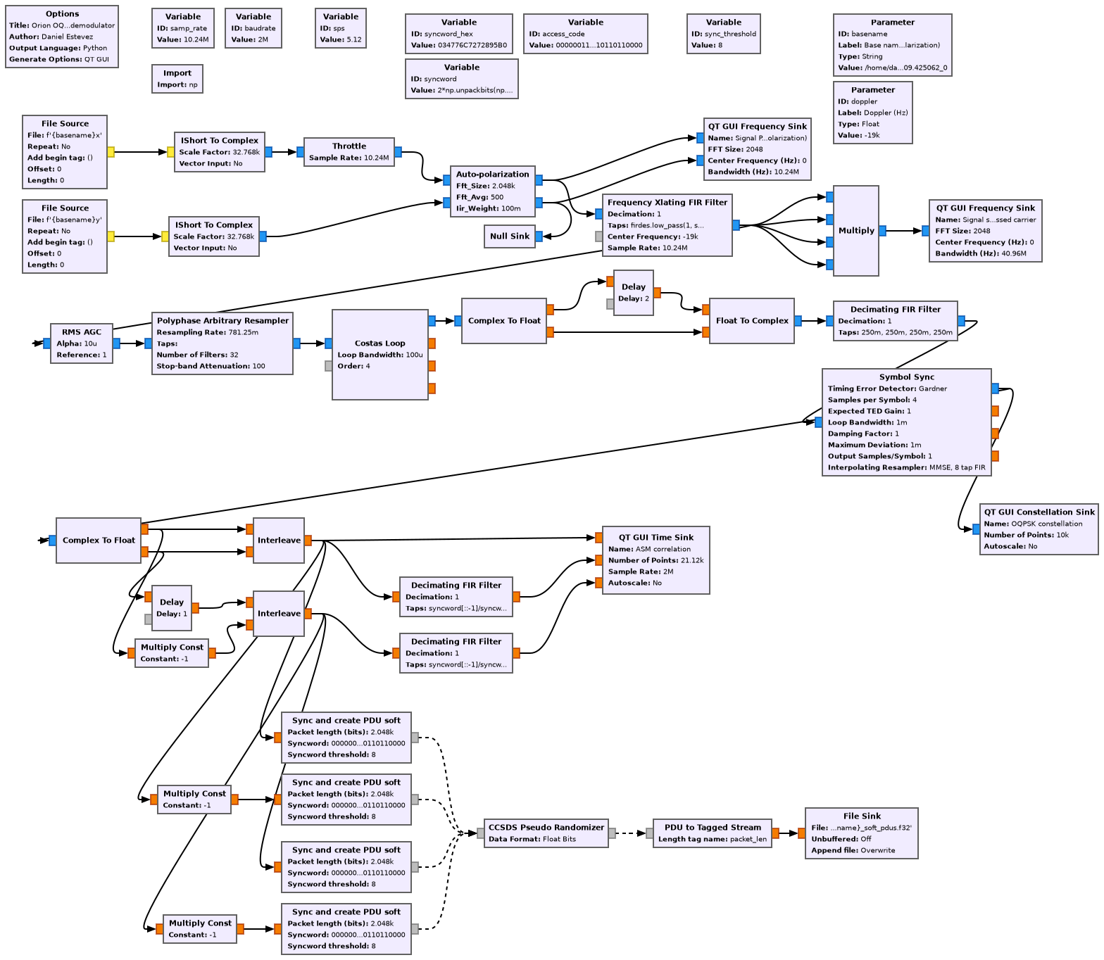
First we use the Auto-polarization block to automatically detect and track the signal polarization. The ATA feeds have vertical and horizontal linear polarization, so we have an input IQ file for each of these polarizations. The Auto-polarization block finds the linear combination of these polarizations that maximizes the SNR (which corresponds to some particular polarization), and gives that at the output, together with the orthogonal polarization. If we see no trace of the signal in the orthogonal polarization, it means that the Auto-polarization block is tracking the polarization correctly. This is an Embedded Python Block that I made a few years ago as a quick prototype. I should really add it to gr-satellites, since I keep re-using it here and there.

The trick of computing the fourth power of the signal is used to find the carrier frequency. This can be used to tune the signal, correcting for Doppler. Since the Costas loop uses a rather narrow bandwidth, it would take too long to lock on its own if the initial error is large.

After the Auto-polarization, there is a Frequency Xlating FIR Filter block that corrects Doppler and leaves only the main lobe of the modulation, to reduce the squaring losses in the Costas loop. Next we have the OQPSK demodulator as described above. Its two output branches (0º and 90º ambiguities) are correlated with the 64-bit ASM used for CCSDS LDPC transfer frames and the results are plotted.

The ASM is found using the Sync and create PDU soft block from gr-satellites, which outputs PDUs containing 2048 soft symbols whenever it sees an ASM (allowing up to a certain maximum number of bit errors in the ASM detection). The frames are descrambled using a block from gr-dslwp, mainly because the gr-satellites CCSDS descrambler only works with hard symbols (another point where we could improve gr-satellites). Finally, the frames are written to a file.

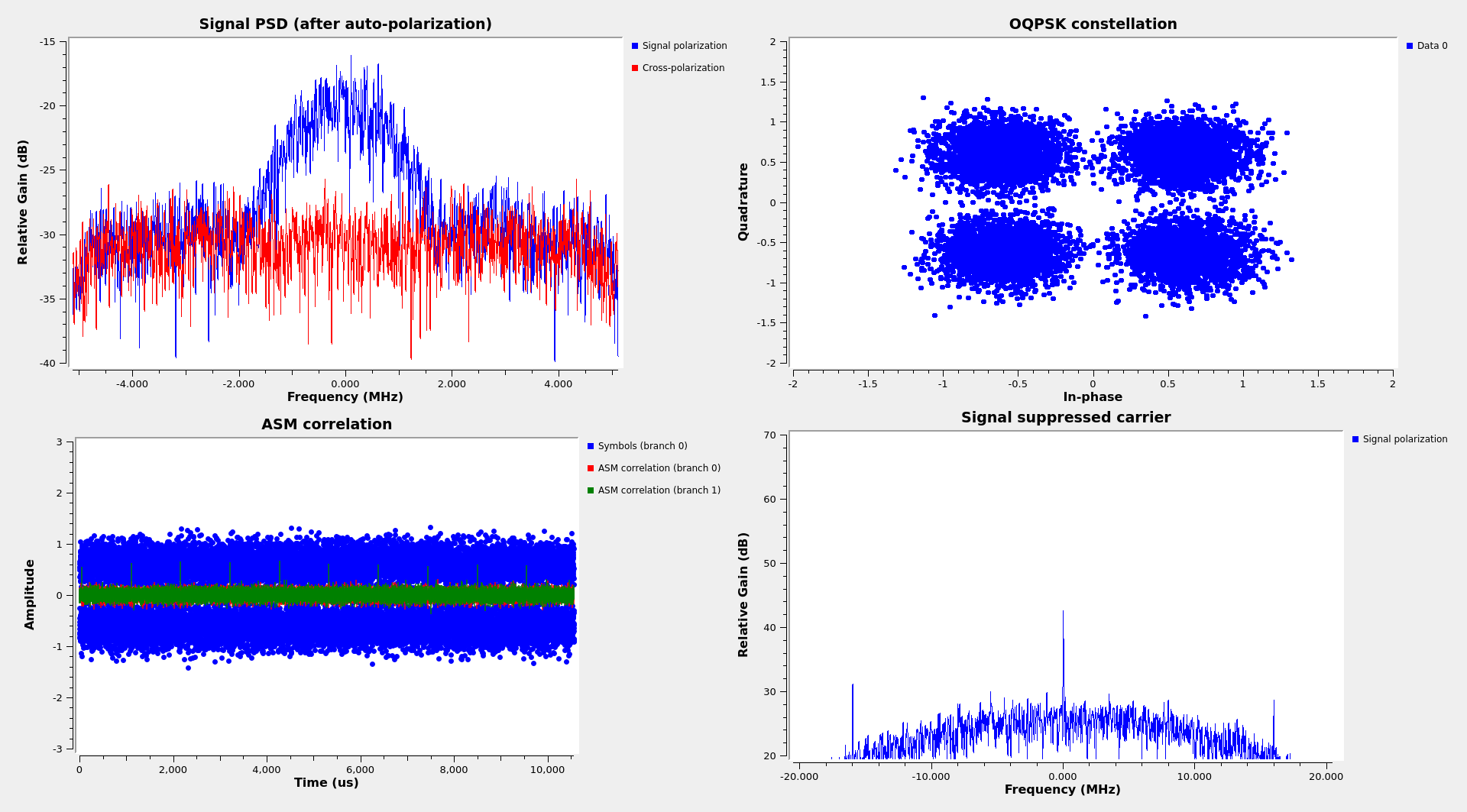
The figure below shows the GUI of the GNU Radio demodulator flowgraph running on one of the ATA recordings. Note that the OQPSK constellation is relatively clean.

LDPC decoding

The CCSDS TM Synchronization and Channel Coding Blue Book defines two “state-of-the-art” FEC systems: Turbo Codes and LDPC codes. Turbo Codes are typically used for deep space applications, while LDPC codes are more popular in near-Earth missions. The Orion vehicle fits more into the near-Earth missions (in the CCSDS nomenclature, it is a Category A spacecraft, because it operates within 2 million km of Earth), so it is logical that it uses LDPC codes.

While for Turbo codes we have some GNU Radio blocks in gr-dslwp (originally developed by Wei Mingchuan BG2BHC using the library deepspace-turbo implemented by Gianluca Marcon), I don’t think there is an openly available GNU Radio implementation of the CCSDS LDPC codes.

Initially I intended to use the LDPC Decoder included in GNU Radio’s FECAPI framework. However I found a couple of issues. First, for some reason I haven’t understood yet, the GNU Radio LDPC decoder was converging to the all zero codeword in 2 iterations, even when given a codeword that has a single bit error (when the codeword is correct it immediately finishes without changing the codeword). Second, the GNU Radio LDPC decoder was taking as systematic bits the wrong bits. The CCSDS LDPC codes use the first \(k\) bits as systematic. However, the GNU Radio LDPC decoder chooses as systematic bits some other bits in general, depending on a construction of a generator matrix described Appendix A.1 of the book Modern Coding Theory, by Richardson and Urbanke.

The second problem is easily fixable by changing this line of the code to get the first \(k\) bits of the estimate instead of using get_systematic_bits(). However, I was clueless about how to solve the first problem in reasonable time.

For this reason I decided to try an alternative and use the library AFF3CT. I have previously shown in this blog how to use AFF3CT to evaluate the performance of LDPC codes, which is the main goal of this library. Though usually AFF3CT is used by means of a command line application that performs an end-to-end simulation with an encoder, modulator, channel model, demodulator and decoder, it is also possible to use it as a C++ library and incorporate some of these blocks into another application. There is a series of example projects that show how this is done.

In any case, to use AFF3CT or the GNU Radio LDPC decoder, it is necessary to have the alist for the code. This is a text file format that describes a sparse matrix. It is intended to describe the parity check matrix of an LDPC code, and most decoders use alists to specify the code to use in this way.

I have a Rust application/library called ldpc-toolbox which already has the ability to generate alists for all the DVB-S2 LDPC codes. Therefore, it made sense to extend this application to support generating alists for the CCSDS LDPC codes. I have added support for all the CCSDS AR4JA codes, as they all use the same kind of protograph construction based on block circulant matrices. In addition to these codes, there is another LDPC code called C2 specified in the TM Synchronization and Coding Blue Book. This is based on a different construction, so I haven’t implemented it.

Starting with one of the AFF3CT application examples, I have made a small tool called aff3ct-ldpc-decoder that reads frames with soft symbols from a binary file and writes decoded frames to a binary file. Currently this only works with the CCSDS r=1/2, k=1024 code, since it has some of the size parameters hardcoded. As it uses an alist (produced with ldpc-toolbox), it should be quite easy to modify it to allow a wider set of LDPC codes.

The LDPC decoder algorithm used by this tool is belief propagation with flooding message passing schedule and the sum-product algorithm. This is probably the most popular LDPC decoding algorithm, and it has good performance. AFF3CT supports a large number of decoding algorithms, so it would be simple to change the tool to use any other of these algorithms. I haven’t taken much care in specifying an accurate noise variance for the calculation of LLRs. In a small piece of one of the ATA recordings I have measured a BER of around 1%. With this relatively low BER, the decoder can works well even without an accurate noise variance estimate.

I haven’t optimized execution speed either. To improve this, I think it’s possible to use SIMD with the sum-product algorithm. Additionally, the decoder should be multithreaded. Right now it runs on a single thread. Currently the decoding speed is about 1/3 of real time in my Ryzen 7 5800X desktop machine and 1/6 of real time in the gnuradio1 machine in the ATA, which has two Xeon Silver 4216 CPUs. Clearly running this as multithreaded would make it much faster than real time, since the Ryzen CPU has 16 cores and the gnuradio1 machine has 64 cores in total.

The CCSDS LDPC codes are actually punctured codes. The protrograph used in the AR4JA construction has some nodes that must be punctured. In the particular case of the r=1/2, k=1024 code, the (2048, 1024) code is obtained by puncturing the last 512 bits from a (2560, 1024) code. In the aff3ct-ldpc-decoder tool, the puncturing is handled by appending 512 zeros to the 2048 soft symbols output by the GNU Radio demodulator and feeding 2560 symbols into the AFF3CT LDPC decoder.

The aff3ct-ldpc-decoder tool can be run as

aff3ct-ldpc-decoder alists/ccsds_ar4ja_r1_2_k1024.alist \
    soft_symbols.f32 frames.u8

At the end of the execution it will print how many frames have been decoded correctly and how many have failed. The CCSDS documents mention that these LDPC codes are very unlikely to give false decodes, so the use of a FECF (frame error control field; CRC-16) is optional. Orion doesn’t use a FECF.

AOS frames

The 128-byte frames transmitted by Orion are AOS Transfer Frames, as described in the CCSDS AOS Space Data Link Protocol Blue Book. The spacecraft ID is 0x14. In the SANA registry, this spacecraft ID is assigned to the spacecraft MPCV, which stands for Multi-Purpose Crewed Vehicle, the official name for Orion. It seems that the same spacecraft ID will be re-used in all the Orion missions.

Only virtual channels 1 and 63 are in use. Virtual channel 1 carries the useful data, which seems to be encrypted. Virtual channel 63 carries only-idle-data, as mandated by CCSDS. There is no Transfer Frame Insert Zone, Operational Control Field or Frame Error Control Field.

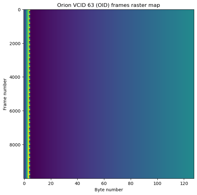
The Transfer Frame Data Field of each idle frame in virtual channel 63 is filled with a counter that ranges from 0x00 to 0x79. This causes a gradient to show up in the raster map of these frames. The plot below shows 10000 frames from VCID 63.

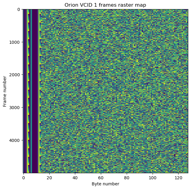
The frames in virtual channel 1 carry encrypted data. It seems that the 4 bytes following the AOS Primary Header always contain 0x81010000. The next 4 bytes contain a counter that increases by one with each frame transmitted in this virtual channel. I think that this field is an IV for the encryption algorithm. It is quite possible that some of the previous four bytes also form part of this counter, perhaps even the whole 8 bytes, giving a 64-bit counter.

The figure below shows the raster map of 10000 frames from virtual channel 1. The IV counter can be seen immediately to the left of the block of 114 bytes of encrypted data, which looks quite random.

An IV shouldn’t be re-used twice with the same key. Therefore, the length of the counter used for the IV should be large enough that it never wraps around. It takes 528 usec to transmit one of these frames. Therefore, a 32-bit counter would take 26 days to wrap. The expected mission duration is 25 days, and the spacecraft doesn’t transmit encrypted data all the time. However, it is quite possible that they have designed the IV counter with more margin, making it 48-bits or 64-bits.

It is interesting to look at the difference between the virtual channel frame count in the AOS Primary Header and this counter. Since both fields increase by one with each frame in virtual channel 1, their difference should stay constant, except for the fact that the virtual channel frame count is only 24-bits wide.

The difference in the recording done on 2022-11-16 at 14:14 UTC was in 0x01040001. The difference in the recording done at 16:22 UTC had jumped to 0x02040001 (it takes 2.46 hours at 100% occupation for the 24-bit counter to wrap around). I find remarkable, but not so surprising, that the 24 least-significant bits differ by a round number as 0x040001. It would be logical that the virtual channel frame counter and the IV counter were reset at the same time at the mission start (or perhaps during pre-flight checks). In this case, the difference between them would be 0x000000. Perhaps the IV counter would be reset to 1 and the frame counter to 0. In this case the difference would be 0x000001. The presence of a 0x04 in the most significant byte is interesting, and I don’t have a good idea to explain it.

Note that this guesswork doesn’t consider resets during flight. Typically we wouldn’t want the IV to reset (to avoid repetition), so it should be backed up by a battery or saved to some kind of non-volatile storage. In contrast, it is not important that the virtual channel frame counter gets reset, so it is quite possible that it resets whenever the spacecraft’s radio is rebooted.

Preliminary results

I have decoded the data in two recordings that were done with the ATA. These IQ recordings used a sample rate of 10.24 Msps and were centred at 2216.5 MHz. The signals from the two linear polarizations from antennas 1a and 5c were recorded. I have only used the data from antenna 1a, using the Auto-polarization block as described above. The two recordings correspond to the following time intervals on 2022-11-16:

• 14:14:20 – 14:54:16 UTC. This recording contains the first outbound correction burn, which happened around 14:33 UTC and lasted for some 30 seconds.
• 16:22:38 – 16:42:54 UTC.

In addition to these two recordings, I made an earlier recording at 20.48 Msps centred at 2210 MHz, but I haven’t processed it yet.

From the first recording, the LDPC decoder could decode 4461508 frames from a total of 4469682, failing to decode 8174 frames. For the second recording, the results were much better. The LDPC decoder could decode 2303286 out of 2303368 frames, failing to decode only 82 frames. These statistics do not take into account frames that could have been skipped because the ASM was not detected.

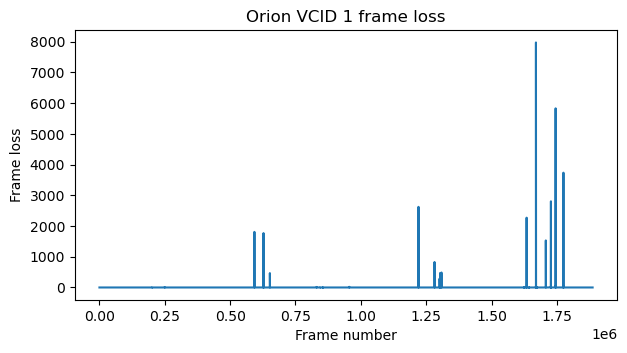
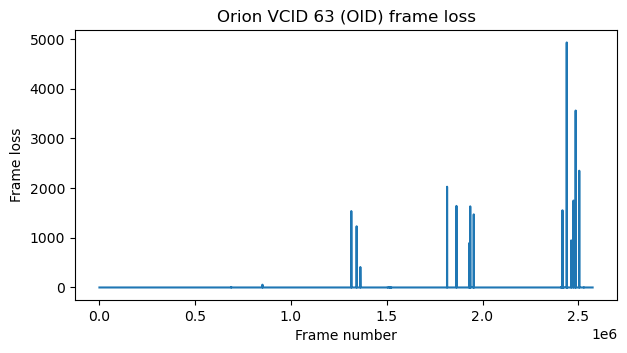
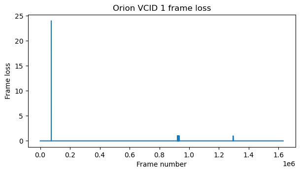
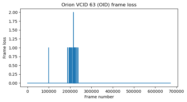
Using the virtual channel frame counters, we see that we lost a total of 77277 frames in the first recording, and only 103 frames in the second recording.

The figures below show the frame loss in each virtual channel during the first recording. We see that there are large spikes were many frames are lost.

The corresponding figures for the second recording are shown here. Only a few frames are lost, but there seem to be some bad bursts. Note that the x-axes of the two figures can’t be directly compared due to the changes in the occupancy rate of each virtual channel.

It is quite possible that the decoder parameters can be tweaked to reduce the number of lost frames. I haven’t even looked a the full waterfalls of these recordings to assess the signal quality and check if there are SNR drops that coincide with the moments when frames are lost. As shown in the spectrum plot at the beginning of the post, the SNR should be good enough for error-free decoding.

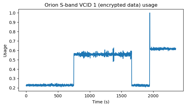
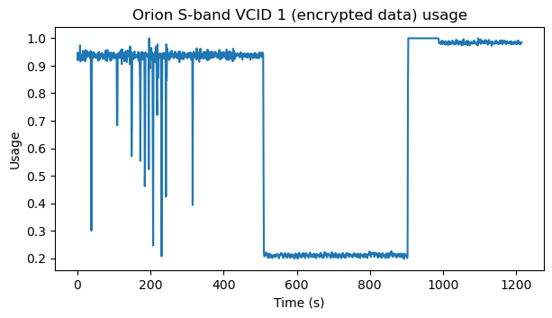
The two figures below show the usage rate of virtual channel 1. This corresponds to the fraction of the link capacity that is occupied with useful data. We can see sudden changes, most likely as the spacecraft responds to commands from ground and changes the types of data that it sends.

Code and data

The GNU Radio flowgraphs and Jupyter notebooks used in this post can be found in this repository. Additionally, the tool aff3ct-ldpc-decoder has been used for LDPC decoding.

Since it will probably take me a while until the ATA recordings are properly reduced, tagged with metadata and published on Zenodo, but I wanted to give people the possibility to play with all this software in the mean time, I have temporarily uploaded a 10 second except taken from the beginning of the second recording (16:22 UTC) to this Google drive folder. This will be deleted when longer recordings (hopefully as long as reasonable) are published in Zenodo.