hf – Page 2 – Daniel Estévez

Waterfalls from the eclipse

Last Monday I did a recording for the HamSci eclipse 2017 HF wideband recording experiment. I used my Hermes-Lite 2.0beta2 to record three 384kHz slices: the 40m band, the 30m band and the 20m band, from 14:00 to 22:00UTC. The 3 band recording in Digital RF format has a size of 248GB, so I’m still compressing the data to upload it to Zenodo.

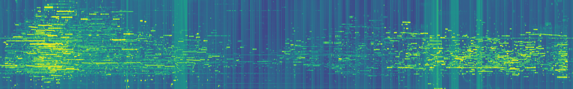
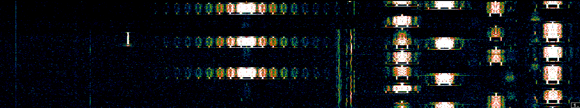
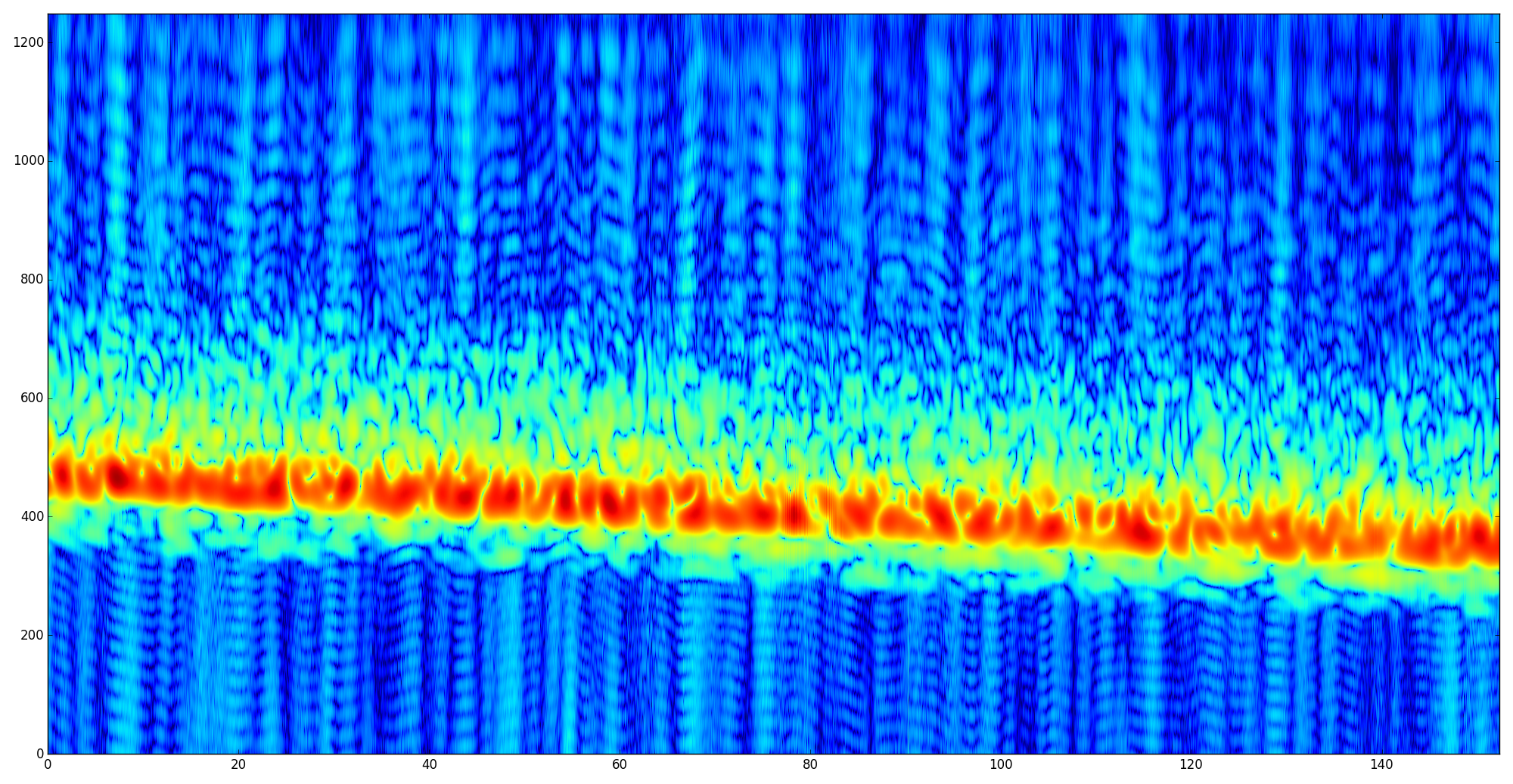
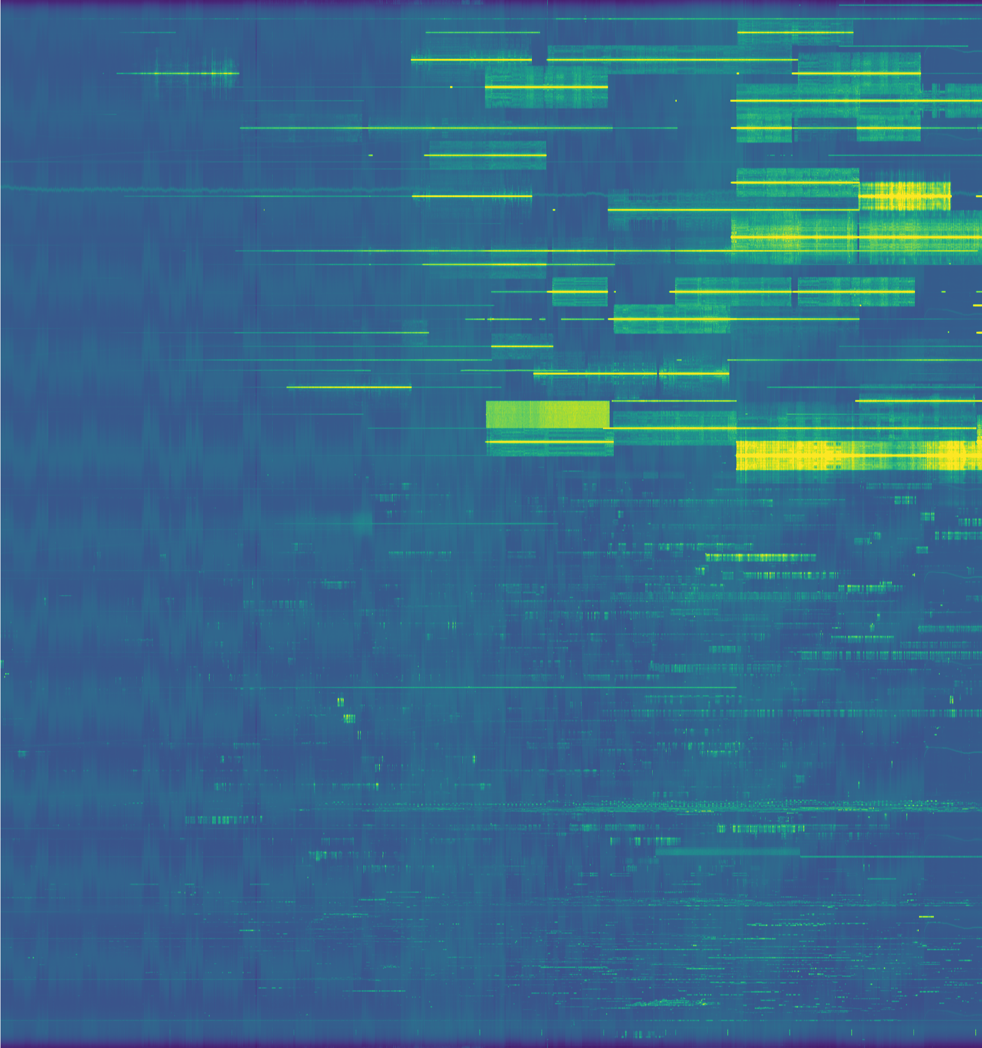
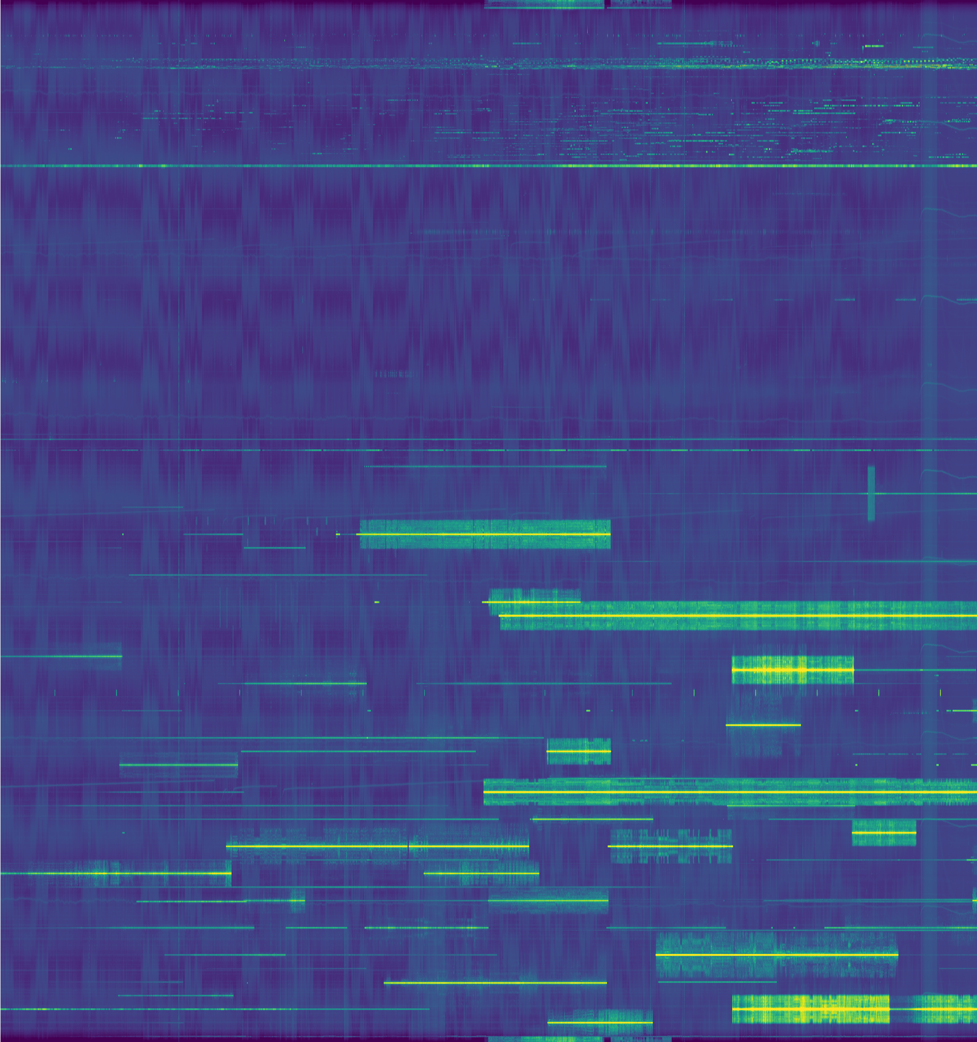
Meanwhile, I have used a variation of my usual Python script to plot waterfalls of the recording. Below you can see waterfalls for the 3 bands. They use the same scaling, with a dynamic range of 50dB, so it is easy to see how the noise floor changes per band. The carriers of the strongest broadcast AM stations are clipped. The resolution in these waterfalls is 187.5Hz or 15s per pixel.

40m waterfall (centre frequency 7180kHz)

30m waterfall (centre frequency 9970kHz)

20m waterfall (centre frequency 14175kHz)

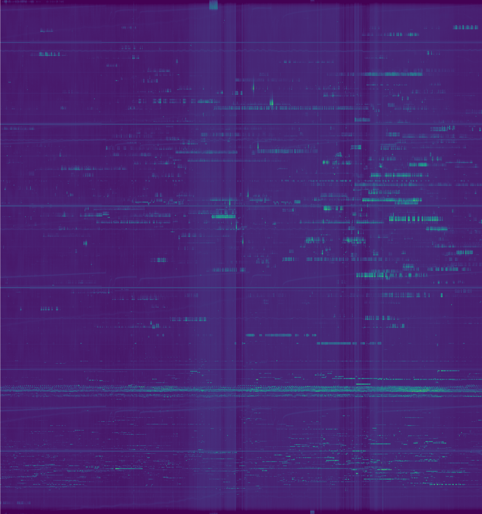
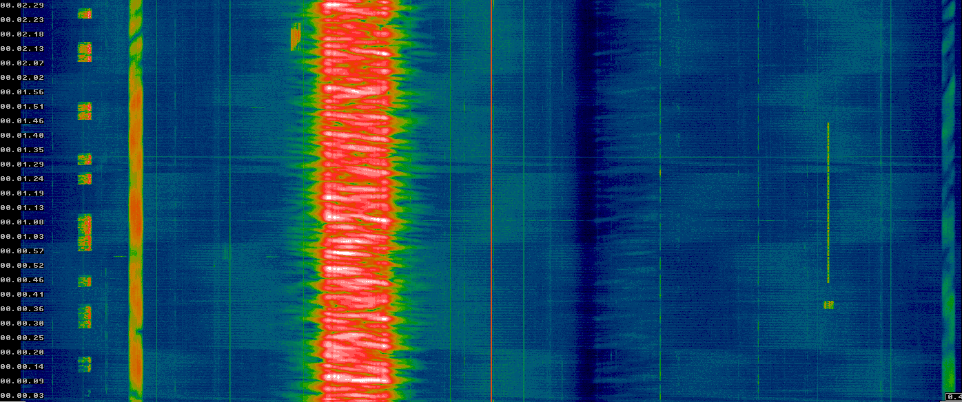
I have also taken a high resolution waterfall around the WWV carrier at 10MHz. The resolution is 22.9mHz or 65.5s per pixel, and the frequency span is 19.95Hz.

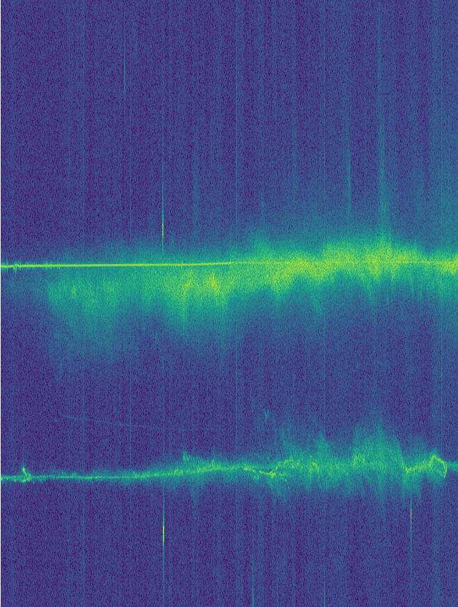
Near the centre of this waterfall, two signal can be seen. The signal which is concentrated in frequency is leakage from my 10MHz GPSDO. The signal which is spread out in frequency is the carrier of WWV, probably mixed with BPM. I’m not sure about the identity of the signal below them, which is about 5Hz below 10MHz. I suspect that it is JN53DV.

This waterfall shows that the 500ppb TCXO of my Hermes-Lite 2.0beta2 is stable to a few tens of parts per billion, as I remarked in my WSPR study.

I have also uploaded large high resolution waterfalls. The Python code used to produce these images is in this gist.

Update 29/08/2017: I have finished uploading the IQ recordings to Zenodo. These are found at:

Waterfalls from the EAPSK63 contest

Last weekend, I recorded the full EAPSK63 contest in the 40m band with the goal of monitoring IMD levels. I made a 48kHz IQ recording spanning the full 24 contest hours (from 16:00 UTC on Saturday to 16:00 UTC on Sunday). This week I’ve been playing with making waterfall plots from the recording. These are very interesting, showing patterns in propagation and contest activity. Here I show some of the waterfalls I’ve obtained, together with the Python code used to compute them.

Monitoring IMD levels in the EAPSK63 contest

This weekend I have recorded the full EAPSK63 Spanish PSK63 contest in the 40m band with the goal of playing back the recording later and reporting the stations showing excessively high IMD levels. In PSK contests, it is usual to see terribly distorted signals, which are the result of reckless operating techniques and stations which are setup inadequately. Contest rules don’t help much, as they are usually too weak to prevent distorted signals from interfering other participants. Amateurs should take care and strive to produce a signal as clean as possible. For instance, in the US, Part 97 101 a) states that “each amateur station must be operated in accordance with good engineering and good amateur practice”. Here I describe the signal processing done in this study and list a “hall of shame” of the worst stations I have spotted in my recording. I will notify by email the contest manager and all the stations in this list with the hope that the situation improves in the future.

Improving signal processing in my OTH radar receiver

This is a follow up post to my experiments studying OTH radar. I have found that the signal processing I did there to obtain the cross-correlation was far from optimal. This produced the strange side-bands below the main reflection. The keen reader might have noticed that I was doing the cross-correlation with a template pulse that lasted the whole pulse repetition cycle. However, the pulses from the radar are shorter. Therefore, it is a better idea to use a shorter template pulse. Ideally, the template pulse should have the same length as the transmitted pulse. However, I don’t know this length precisely, because multipath propagation makes the received pulses a bit longer. However, I think that 6.5ms is a good estimate.

I have also changed the window for the pulse. I’m now using a Dolph-Chebyshev window. I use scipy to compute this window, because it is not included in GNU Radio. This window has the property that the side-bands have constant attenuation. Indeed, it minimizes the \(L^\infty\) norm of the side-bands. There is a parameter that tunes the side-bands attenuation. For higher attenuations, you have a wider main lobe, while if you want a narrower main love you get less side-band attenuation. These properties make this window useful in radar applications.

Below I’m doing the cross-correlation in GNU Radio with a shorter template pulse shaped with a Dolph-Chebyshev window set for 55dB attenuation.

The good thing about the settable attenuation of the Dolph-Chebyshev window is that it can be used to trade-off performance between different features. First, we use an attenuation of 100dB. The side-bands are below the noise floor in this case, so we have no “false responses” in our cross-correlation. The drawback is that the main lobe is wide so the resolution of the features of the ionosphere in the image below is not very good.

Dolph-Chebyshev window with 100dB attenuation

Next we try with 55dB attenuation. This narrows the main lobe, improving the resolution and crispness of the features of the ionosphere in the image below. However, side-bands start being visible above the noise floor, producing “false responses”. However, comparing with the image above, we now know where the false responses are.

Dolph-Chebyshev window with 55dB attenuation

I have updated the gist with the GNU Radio flowgraph and python script used to produce the images.

Looking at an HF OTH radar

Most amateur operators are familiar with over-the-horizon radars in the HF bands. They sometimes pop up in the Amateur bands, rendering several tens of kilohertzs unusable. Inspired by Balint Seeber’s talk in GRCon16, I’ve decided to learn more about radars. Here I look at a typical OTH radar, presumably of Russian origin. It was recorded at my station around 20:00UTC on 8 December at a frequency around 6860kHz. This radar sometimes appears inside the 40m Amateur band as well.

Listening to the FreeDV net by WebSDR

Since I’m away from my usual QTH, I decided to join yesterday’s FreeDV net by listening through the University of Twente WebSDR and giving signal reports on the QSO Finder to the stations transmitting.