Amateur radio – Page 2 – Daniel Estévez

DVB-S2 GRCon23 CTF challenge

This year I submitted a challenge track based around a DVB-S2 signal to the GRCon CTF (see this post for the challenges I sent in 2022). The challenge description was the following.

I was scanning some Astra satellites and found this interesting signal. I tried to receive it with my MiniTiouner, but it didn’t work great. Maybe you can do better?

Note: This challenge has multiple parts, which can be solved in any order. The flag format is flag{...}.

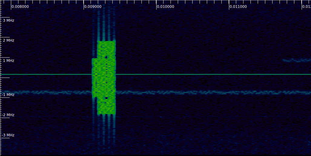
A single SigMF recording with a DVB-S2 signal sampled at 2 Msps at a carrier frequency of 11.723 GHz was given for the 10 flags of the track. The description and frequency were just some irrelevant fake backstory to introduce the challenge, although some people tried to look online for transponders on Astra satellites at this frequency.

The challenge was inspired by last year’s NTSC challenge by Clayton Smith (argilo), which I described in my last year’s post. This DVB-S2 challenge was intended as a challenge with many flags that can be solved in any order and that try to showcase many different places where one might sensibly put a flag in a DVB-S2 signal (by sensibly I mean a place that is actually intended to transmit some information; surely it is also possible to inject flags into headers, padding, and the likes, but I didn’t want to do that). In this sense, the DVB-S2 challenge was a spiritual successor to the NTSC challenge, using a digital and modern TV signal.

Another source of motivation was one of last year’s Dune challenges by muad’dib, which used a DVB-S2 Blockstream Satellite signal. In that case demodulating the signal was mostly straightforward, and the fun began once you had the transport stream. In my challenge I wanted to have participants deal with the structure of a DVB-S2 signal and maybe need to pull out the ETSI documentation as a help.

I wanted to have flags of progressively increasing difficulty, keeping some of the flags relatively easy and accessible to most people (in any case it’s a DVB-S2 signal, so at least you need to know which software tools can be used it to decode it and take some time to set them up correctly). This makes a lot of sense for a challenge with many flags, and in hindsight most of the challenges I sent last year were quite difficult, so I wanted to have several easier flags this time. I think I managed well in this respect. The challenge had 10 flags, numbered more or less in order of increasing difficulty. Flags #1 through #8 were solved by between 7 and 11 teams, except for flag #4, which was somewhat more difficult and only got 6 solves. Flags #9 and #10 were significantly more difficult than the rest. Vlad, from the Caliola Engineering LLC team, was the only person that managed to get flag #10, using a couple of hints I gave, and no one solved flag #9.

When I started designing the challenge, I knew I wanted to use most of the DVB-S2 signal bandwidth to send a regular transport stream video. There are plenty of ways of putting flags in video (a steady image, single frames, audio tracks, subtitles…), so this would be close to the way that people normally deal with DVB-S2, and give opportunities for many easier flags. I also wanted to put in some GSE with IP packets to show that DVB-S2 can also be used to transmit network traffic instead of or in addition to video. Finally, I wanted to use some of the more fancy features of DVB-S2 such as adaptive modulation and coding for the harder flags.

To ensure that the DVB-S2 signal that I prepared was not too hard to decode (since I was putting more things in addition to a regular transport stream), I kept constantly testing my signal during the design. I mostly used a Minitiouner, since perhaps some people would use hardware decoders. I heard that some people did last year’s NTSC challenge by playing back the signal into their hotel TVs with an SDR, and for DVB-S2 maybe the same would be possible. Hardware decoders tend to be more picky and less flexible. I also tested gr-dvbs2rx and leandvb to have an idea of how the challenge could be solved with the software tools that were more likely to be used.

What I found, as I will explain below in more detail, is that the initial way in which I intended to construct the signal (which was actually the proper way) was unfeasible for the challenge, because the Minitiouner would completely choke with it. I also found important limitations with the software decoders. Basically they would do some weird things when the signal was not 100% a regular transport stream video, because other cases were never considered or tested too thoroughly. Still, the problems didn’t get too much in the way of getting the video with the easier flags, and I found clever ways of getting around the limitations of gr-dvbs2rx and leandvb to get the more difficult flags, so I decided that this was appropriate for the challenge.

In the rest of this post I explain how I put together the signal, the design choices I made, and sketch some possible ways to solve it.

Demodulation of the 5G NR downlink

At the end of July, Benjamin Menkuec was commenting in Twitter about some issues he had while demodulating a 5G NR downlink recording. There was a lively discussion in which other people and I participated. I had never touched 5G, but had done some work with LTE, so I decided to take the chance to learn more about the 5G physical layer. Compared to LTE, the changes are more evolutionary than revolutionary, but understanding what has changed, and how and why, is part of the puzzle.

I had to take an 11.5 hour flight in a few days, so I thought it would be a nice challenge to give this a shot, take with me the recordings that Benjamin was using and all the 3GPP documents, and write a demodulator in a Jupyter notebook from scratch during the flight, as I had done in the past with my LTE recordings. This turned out to be an enjoyable and interesting experience, quite different from working at home in shorter intervals scattered over multiple days or weeks, and with internet access. At the end of the flight I had a mostly working demodulation, but it had a few weird problems that turned out to be caused by some mistakes and misconceptions. I worked on cleaning this up and solving the problems over the next few days, and also now preparing this post.

Rather than trying to give an account of all my mistakes and dead ends (I spoke a little about these in Twitter), in this post I will show the final clean solution. There are some tricky new aspects in 5G NR (phase compensation, as we will see below) which can be quite confusing, so hopefully this post will do a good job at explaining them in a simple way.

The Jupyter notebook used in this post is here, and the recording in SigMF format can be found in this folder. Here I will only be using the first of Benjamin’s two recordings, since they are quite similar. It was done with an ADALM Pluto at 7.86 Msps and has a duration of 143 ms. The transmitter is an srsRAN 5 MHz cell. The recording was done off-the-air, or maybe with a cabled set up, but there are some other signals leaking in. The SNR is very good, so this is not a problem.

The first signal we find is at 9 ms. There is a transmission like this every 10 ms. As we will see, this is an SS/PBCH block. Something that stands out to those familiar with the LTE downlink spectrum is that the 5G NR spectrum is almost empty. In LTE, the cell-specific reference signals are transmitted all the time. In 5G this is not the case. Downlink signals are transmitted only when there is traffic. There is always a burst of one or several SS/PBCH blocks transmitted periodically (usually every 20 ms, but in this recording every 10 ms), as well as other signals that are always sent periodically (such as the SIB1 in the PDSCH), but this may be all if there is no traffic in the cell.

A very quick RFI survey at the Allen Telescope Array

At the beginning of August I visited the Allen Telescope Array (ATA) for the Breakthrough Listen REU program field trip (I have been collaborating with the REU program for the past few years). One of the things I did during my visit was to use an ADALM Pluto running Maia SDR to do a very quick scan of the radio frequency interference (RFI) on-site. This was not intended as a proper study of any sort (for that we already have the Hat Creek Radio Observatory National Dynamic Radio Zone project), but rather as a spoor-of-the-moment proof of concept.

The idea was to use equipment I had in my backpack (the Pluto, a small antenna, my phone and a USB cable), step just outside the main office, scroll quickly through the spectrum from 70 MHz to 6 GHz, stop when I saw any signals (hopefully not too many, since Hat Creek Radio Observatory is supposed to be a relatively quiet radio location), and make a SigMF recording of each of the signals I found. It took me about 15 minutes to do this, and I made 6 recordings in the process. A considerable amount of time was spent downloading the recordings to my phone, which takes about one minute per recording (since recordings are stored on the Pluto DDR, only one recording can be stored on the Pluto at a time, and it must be downloaded to the phone before making a new recording).

This shows that Maia SDR can be a very effective tool to get a quick idea of how the local RF environment looks like, and also to hunt for local RFI in the field, since it is quite easy to carry around a Pluto and a phone. The antenna I used was far from ideal: a short monopole for ~450 MHz, shown in the picture below. This does a fine job at receiving strong signals regardless of frequency, but its sensitivity is probably very poor outside of its intended frequency range.

The following plot shows the impedance of the antenna measured with a NanoVNA V2. The impedance changes noticeably if I put my hand on the NanoVNA, with the resonant peak shifting down in frequency by 50 to 100 MHz. Therefore, this measurement should be taken just as a rough ballpark of how the antenna looks like on the Pluto, which I was holding with my hand.

As the antenna I used for this survey is pretty bad, the scan will only show signals that are actually very strong on the ATA dishes. The log-periodic feeds on the ATA dishes tend to pick up signals that do not bounce off the dish reflectors, and instead arrive to the feed directly from a side. This is different from a waveguide type feed, in which signals need to enter through the waveguide opening. Therefore, besides having the main lobe corresponding to a 6.1 m reflector, the dishes also have relatively strong sidelobes in many directions, with a gain roughly comparable to an omnidirectional antenna. The system noise temperature of the dishes is around 100 to 150 K (including atmospheric noise and spillover), while the noise figure of the Pluto is probably around 5 dB. This all means that the dishes are more sensitive to detect signals from any direction that the set up I was using. In fact, signals from GNSS satellites from all directions can easily be seen with the dishes several dB above the noise floor, but not with this antenna and the Pluto.

Additionally, the scan only shows signals that are present all or most of the time, or that I just happened to come across by chance. This quick survey hasn’t turned up any new RFI signals. All the signals I found are signals we already knew about and have previously encountered with the dishes. Still, it gives a good indication of what are the strongest sources of RFI on-site. Something else to keep in mind is that the frequency range of the Allen Telescope Array is usually taken as 1 – 12 GHz. Although the feeds probably work with some reduced performance somewhat below 1 GHz, observations are done above 1 GHz. Therefore, none of the signals I have detected below 1 GHz are particularly important for the telescope observations, since they are not strong enough to cause out-of-band interference.

I have published the SigMF recordings in the Zenodo dataset Quick RFI Survey at the Allen Telescope Array. All the recordings have a sample rate of 61.44 Msps, since this is what I was using to view the largest possible amount of spectrum at the same time, and a duration of 2.274 seconds, which is what fits in 400 MiB of the Pluto DDR when recording at 61.44 Msps 12 bit IQ (this is the maximum recording size for Maia SDR). The published files are as produced by Maia SDR. At some point it could be interesting to add additional metadata and annotations.

In the following, I do a quick description of each of the 6 recordings I made.

ldpc-toolbox gets LDPC decoding

Recently I have implemented an FPGA LDPC decoder for a commercial project. The belief propagation LDPC decoder algorithm admits many different approximations in the arithmetic, and other tricks that can be used to trade off between decoding sensitivity (BER versus Eb/N0 performance) and computational complexity. To help me benchmark the different belief propagation algorithms, I have extended my ldpc-toolbox project to implement many different LDPC decoding algorithms and perform BER simulations.

ldpc-toolbox is a Rust library and command line tool for the design of LDPC codes. I initially created this project when I was trying to design a suitable LDPC code for a narrowband 32APSK modem to be used over the QO-100 amateur GEO transponder. The tool so far supported some classical pseudorandom constructions of LDPC codes, computed Tanner graph girths, and could construct the alists for all the DVB-S2 and CCSDS LDPC codes. Extending this tool to support LDPC encoding, decoding and BER simulation is a natural step.

An erasure FEC for SSDV

SSDV is an amateur radio protocol that is used to transmit images in packets, in a way that is tolerant to packet loss. It is based on JPEG, but unlike a regular JPEG file, where losing even a small part of the file has catastrophic results, in SSDV different blocks of the image are compressed independently. This means that packet loss affects only the corresponding blocks, and the image can still be decoded and displayed, albeit with some missing blocks.

SSDV was originally designed for transmission from high-altitude balloons (see this reference for more information), but it has also been used for some satellite missions, including Longjiang-2, a Chinese lunar orbiting satellite.

Even though SSDV is tolerant to packet loss, to obtain the full image it is necessary to receive all the packets that form the image. If some packets are lost, then it is necessary to retransmit them. Here I present an erasure FEC scheme that is backwards-compatible with SSDV, in the sense that the first packets transmitted by this scheme are identical to the usual \(k\) packets of standard SSDV, and augments the transmission with FEC packets in such a way that the complete image can be recovered from any set of \(k\) packets (so there is no encoding overhead). The FEC packets work as a fountain code, since it is possible to generate up to \(2^{16}\) packets, which is a limit unlikely to be reached in practice.

More about the QO-100 WB transponder power budget

Last week I wrote a post with a study about the QO-100 WB transponder power budget. After writing this post, I have been talking with Dave Crump G8GKQ. He says that the main conclusions of my study don’t match well his practical experience using the transponder. In particular, he mentions that he has often seen that a relatively large number of stations, such as 8, can use the transponder at the same time. In this situation, they “rob” much more power from the beacon compared to what I stated in my post.

I have looked more carefully at my data, specially at situations in which the transponder is very busy, to understand better what happens. In this post I publish some corrections to my previous study. As we will see below, the main correction is that the operating point of 73 dB·Hz output power that I had chosen to compute the power budget is not very relevant. When the transponder is quite busy, the output power can go up to 73.8 dB·Hz. While a difference of 0.8 dB might not seem much, there is a huge difference in practice, because this drives the transponder more towards saturation, decreasing its gain and robbing more output power from the beacon to be used by other stations.

I want to thank Dave for an interesting discussion about all these topics.

Measuring the QO-100 WB transponder power budget

The QO-100 WB transponder is an S-band to X-band amateur radio transponder on the Es’hail 2 GEO satellite. It has about 9 MHz of bandwidth and is routinely used for transmitting DVB-S2 signals, though other uses are possible. In the lowermost part of the transponder, there is a 1.5 Msym QPSK 4/5 DVB-S2 beacon that is transmitted continuously from a groundstation in Qatar. The remaining bandwidth is free to be used by all amateurs in a “use whatever bandwidth is free and don’t interfere others” basis (there is a channelized bandplan to put some order).

From the communications theory perspective, one of the fundamental aspects of a transponder like this is how much output power is available. This sets the downlink SNR and determines whether the transponder is in the power-constrained regime or in the bandwidth-constrained regime. It indicates the optimal spectral efficiency (bits per second per Hz), which helps choose appropriate modulation and FEC parameters.

However, some of the values required to do these calculations are not publicly available. I hear that the typical values which would appear in a link budget (maximum TWTA output power, output power back-off, antenna gain, etc.) are under NDA from MELCO, who built the satellite and transponders.

I have been monitoring the WB transponder and recording waterfall data of the downlink with my groundstation for three weeks already. With this data we can obtain a good understanding of the transponder behaviour. For example, we can measure the input power to output power transfer function, taking advantage of the fact that different stations with different powers appear and disappear, which effectively sweeps the transponder input power (though in a rather chaotic and uncontrollable manner). In this post I share the methods I have used to study this data and my findings.

Monitoring the QO-100 WB transponder usage with Maia SDR

I am interested in monitoring the usage of the QO-100 WB transponder over several weeks or months, to obtain statistics about how full the transponder is, what bandwidths are used, which channels are occupied more often, etc., as well as statistics about the power of the signals and the DVB-S2 beacon. For this, we need to compute and record to disk waterfall data for later analysis. Maia SDR is ideal for this task, because it is easy to write a Python script that configures the spectrometer to a low rate, connects to the WebSocket to fetch spectrometer data, performs some integrations to lower the rate even more, and records data to disk.

For this project I’ve settled on using a sample rate of 20 Msps, which covers the whole transponder plus a few MHz of receiver noise floor on each side (this will be used to calibrate the receiver gain) and gives a frequency resolution of 4.9 kHz with Maia SDR’s 4096-point FFT. At this sample rate, I can set the Maia SDR spectrometer to 5 Hz and then perform 50 integrations in the Python script to obtain one spectrum average every 10 seconds.

Part of the interest of setting up this project is that the Python script can serve as an example of how to interface Maia SDR with other applications and scripts. In this post I will show how the system works and an initial evaluation of the data that I have recorder over a week. More detailed analysis of the data will come in future posts.

Running the AD9361 at 122.88 Msps

The Analog Devices AD9361 is an RFIC that is used in several popular SDRs, such as the USRP B2xx series and E3xx series, the BladeRF 2.0 micro, the ADALM Pluto, the ANTSDR, and in many other products (some of these use the AD9363 or the AD9364, which are similar chips in the same family). This RFIC has a nominal maximum sample rate of 61.44 Msps, and an analog bandwidth of 56 MHz.

A few days ago, Nuand has published a new software version that allows running the BladeRF 2.0 at 122.88 Msps. This has attracted some interest in Twitter, specially regarding questions about how they manage to achieve this and how good the performance is. One of the changes that Nuand has done to support the 122.88 Msps mode is an 8-bit wire protocol for the USB 3.0 interface. This is required to be able to pass 122.88 Msps through the USB. This change affects the FPGA gateware and host drivers. The other change involves manually setting some registers of the AD9361 in the host drivers in order to bypass a half-band filter, effectively doubling the output sample rate. In this post I will give a short review of the AD9361 register settings that enable the 122.88 Msps mode.

Maia SDR

I’m happy to announce the release of Maia SDR, an open-source FPGA-based SDR project focusing on the ADALM Pluto. The first release provides a firmware image for the Pluto with the following functionality:

Web-based interface that can be accessed from a smartphone, PC or other device.
Real-time waterfall display supporting up to 61.44 Msps (limit given by the AD936x RFIC of the Pluto).
IQ recording in SigMF format, at up to 61.44 Msps and with a 400 MiB maximum data size (limit given by the Pluto RAM size). Recordings can be downloaded to a smartphone or other device.