This is a follow-up on the series about DSLWP-B’s orbital dynamics (see part I and part II). In part I we looked at the tracking files published by Wei Mingchuan BG2BHC, which list the position and velocity of the satellite in ECEF coordinates, and presented basic orbit propagation with GMAT. In part II we explored GMAT’s capabilities to plan and perform manoeuvres, making a tentative simulation of DSLWP-B’s mid-course correction and lunar orbit injection. Now we turn to the study of DSLWP-B’s elliptical lunar orbit.
In this post we will examine the Keplerian elements of the orbits described by each of the tracking files published so far. We will also use Scott Tilley VE7TIL’s Doppler measurements of the S-band beacon of DSLWP-B to validate and determine the orbit.
New tracking files get published by Wei in the dslwp_dev Github repository. The HEAD of the master branch only contains the more recent tracking files, but older files can be extracted from the git commit history. So far, the following tracking files have been published:
program_tracking_dslwp-a_20180520_window1.txt
program_tracking_dslwp-b_20180526.txt
program_tracking_dslwp-b_20180528.txt
program_tracking_dslwp-b_20180529.txt
program_tracking_dslwp-b_20180531.txt
program_tracking_dslwp-b_20180601.txt
program_tracking_dslwp-b_20180602.txt
program_tracking_dslwp-b_20180603.txt
The first of them describes the path from Earth to Moon, right after trans-lunar injection, and it has already been examined in part I and part II of this series. The remaining files describe the lunar orbit of DSLWP-B, starting with different epochs. Here we will look at these seven tracking files.
To examine the tracking files and determine if there are any noticeable changes between the orbits described by each of them, we use GMAT to propagate the orbit and compute Keplerian state elements for each file. As we did in part I, the first row of each tracking file is taken as the state of the spacecraft, and then the orbit is propagated first backwards until 2018-05-26 and then forwards for 10 days. The resulting Keplerian elements are plotted in Jupyter for comparison.
The calculations have been performed using this Jupyter notebook.
The plots below show the evolution of the semi-major axis and the mean anomaly for each of the tracking files. These are the orbital elements where differences in the orbit can be seen best.
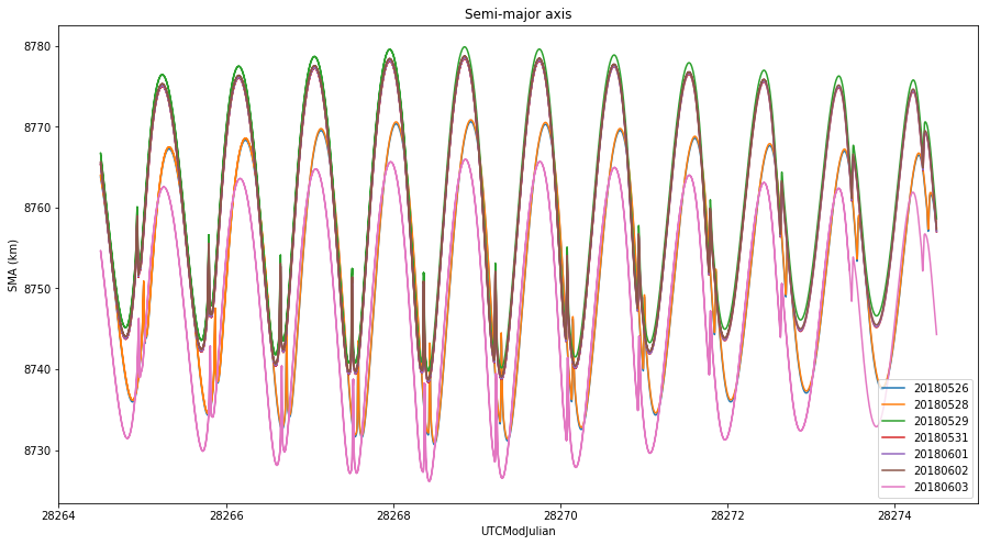

The first thing we notice is that there is a mismatch in the mean anomaly. In the first two tracking files the mean anomaly is shifted in time roughly 1 hour and 46 minutes with respect to the remaining tracking files. This means that the first two tracking files predict that the time of periapsis is 1 hour and 46 minutes later than what the remaining tracking files imply. I already observed this in my preliminary analysis of Scott Tilley’s Doppler measurements and Wei commented that he had made a mistake when producing these two tracking files.
This is interesting because I had calculated the time of periapsis for lunar orbit in part II to be 2018-05-25 16:04:08 UTC, but this didn’t match too well the fact that injection presumably happened around 14:00 or 15:00 UTC. If we factor in this 1 hour and 46 minutes error, then the corrected time of periapsis matches the injection time much better. I leave as an exercise for the reader to redo the calculations in part II with the improved orbital parameters derived in this post.
If we look at the semi-major axis, we can make three groups of tracking files according to their behaviour. The first group is formed by the first two tracking files, with a semi-major axis that peaks at 8770km. The second group is formed by the tracking files 3 to 6, with a semi-major axis that peaks at 8780km (also note that the third tracking file is a little bit different from the rest). The third group is formed only by the last tracking file, with a semi-major axis that peaks at 8765km. We will comment on this difference later.
Another interesting thing to note is that there is some weird thing happening with the semi-major axis at periapsis. This kind of thing was first observed by Jonathan McDowell in the first tracking files describing the lunar orbit. I think I still haven’t understood well this phenomenon. Here the force model I have used for orbit propagation is a detailed model including lunar spherical harmonics up to degree and order 10 and point forces for the Sun and all the planets (except for Mercury and Pluto).
Now we turn to the analysis of Scott Tilley’s Doppler measurements. We take the tracking file from 20180531 as a reference for the orbit of DSLWP-B and use GMAT to simulate the Doppler, as received by Scott’s station.
GMAT has advanced features to simulate two-way Doppler, as produced when transmitting a carrier from a groundstation on Earth to a spacecraft’s transponder and back to another groundstation on Earth (see the tutorial on simulating DSN Range and Doppler data). This simulation includes effects such as the finite propagation speed of light, relativistic corrections, and ionospheric and tropospheric delays. However, there doesn’t seem to be such an advanced system to simulate one-way Doppler such as the one produced by observing DSLWP-B’s beacon from a groundstation on Earth.
Probably the closest we can get to simulate one-way Doppler with GMAT is to use GMAT’s simulation capabilities to measure two-way range-rate with speed of light and relativistic corrections disabled and divide the resulting range-rate by two to obtain the one-way range-rate. This two-way range-rate does its calculations as follows. Let \(R(t)\) denote the two-way range from the groundstation to the spacecraft at time \(t\), so that \(R(t) = 2r(t)\), where \(r(t)\) is the distance between the groundstation and the spacecraft at time \(t\). The two-way range-rate at time \(t\) is computed as \((R(t) – R(t-\delta))/\delta\), where \(\delta\) is known as the Doppler averaging interval. Dividing this two-way range-rate by two we get \((r(t) – r(t-\delta))/\delta\), which is the average value for the Doppler, ignoring relativistic effects and the finite propagation speed of light. Since the propagation time from the Moon to Earth is a bit over one second, it is not so important to consider the propagation time in these simulations, but it would be very important for interplanetary missions.
Another more simple way to calculate Doppler is to make GMAT output the position \(x(t)\) and velocity \(v(t)\) of DSLWP-B in a reference frame centred on Scott’s station. Then we can compute the Doppler as\[\frac{d}{dt}\|x(t)\| = \frac{\langle v(t), x(t)\rangle}{\|x(t)\|}.\]This ignores the relativistic effects, the propagation speed of light, and also the fact that Doppler is measured by averaging over a time interval. However, for short averaging times this calculation is a reasonable approximation.
We use GMAT to simulate Doppler using both approaches and plot the results together with the Doppler measurements by Scott Tilley. To get a good match, we have needed to shift down the Doppler measurements by 3400Hz. Probably this is caused by DSLWP-B’s S-band beacon not being precisely on its nominal frequency of 2275.222MHz (other people list 2275.224MHz as the nominal frequency).
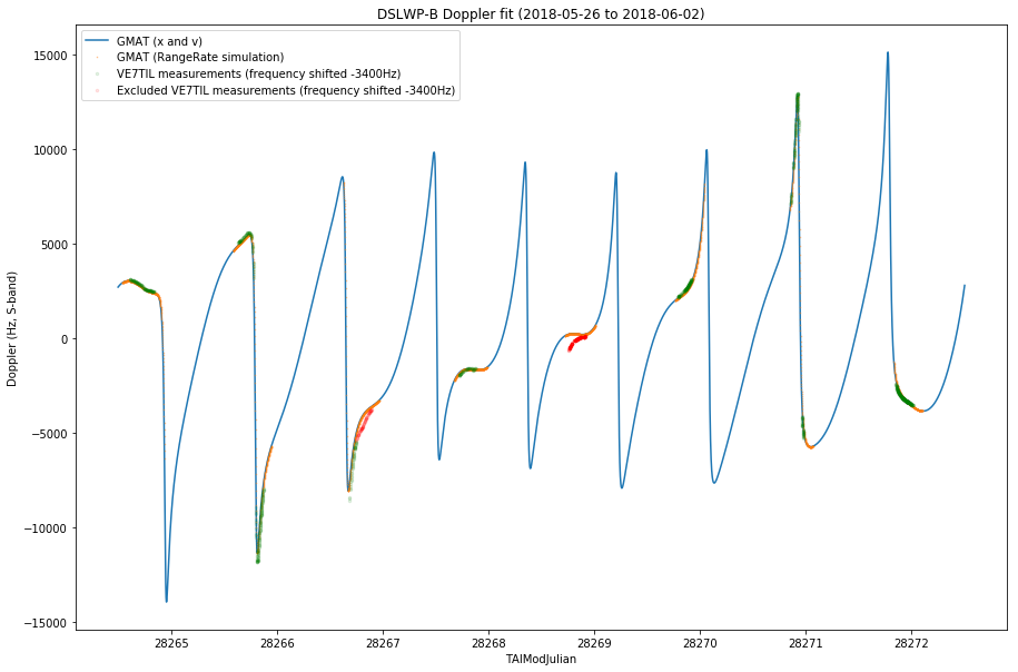
Note that GMAT’s simulation using RangeRate only outputs data whenever DSLWP-B is visible from Scott’s station, while the simple method using \(x\) and \(v\) outputs data for all times.
We see that most of the data measured by Scott matches the simulation rather well. However, there are two time intervals where the match is not good. These probably indicate a frequency drift in DSLWP-B’s beacon (or perhaps in Scott’s receiver) and have been discarded for further analysis. Discarded points are marked in the graph above in red.
This also indicates that the orbital parameters derived from the 20180531 tracking file are more or less accurate. When I analysed the tracking file 20180526 I obtained a large discrepancy, due to an incorrect anomaly at epoch. It also indicates that the drift of the S-band beacon of DSLWP-B is sufficiently low that orbit determination using this data is possible.
Now we use GMAT’s orbit determination capabilities to refine the orbital parameters using Scott’s data. I suggest the reader to take a look at the orbit estimation tutorial.
We use the following initial state for the orbit determination, which has been generated by propagating the 20180531 tracking file.
DSLWP_B.Epoch = '28264.5';
DSLWP_B.SMA = 8765.409054517644;
DSLWP_B.ECC = 0.7618824709853163;
DSLWP_B.INC = 20.80912899224475;
DSLWP_B.RAAN = 307.3706391221838;
DSLWP_B.AOP = 118.7406568683716;
DSLWP_B.TA = 178.2429103785479;
As an error model for the Doppler measurements we use a \(\sigma\) of 0.003km/s, which corresponds to a Doppler shift of around 20Hz. This seems to be approximately the resolution of Scott’s measurements.
The orbit estimation converges, giving the following output:
Estimation converged!
      |1 - RMSP/RMSB| = | 1- 3.49511 / 3.49512| = 2.12288e-06 is less than RelativeTol, 0.0001

Final Estimated State:

   Estimation Epoch:
   28264.5004286386756575666368 A.1 modified Julian
   28264.5004282407393149740443 TAI modified Julian
   26 May 2018 00:00:00.000 UTCG
   DSLWP_B.LunaInertial.SMA = 8761.0758581
   DSLWP_B.LunaInertial.ECC = 0.768016853537
   DSLWP_B.LunaInertial.INC = 16.9728174682
   DSLWP_B.LunaInertial.RAAN = 295.670653562
   DSLWP_B.LunaInertial.AOP = 130.427472407
   DSLWP_B.LunaInertial.TA = 178.126596496

Final Covariance Matrix:

         2.775051914396e-04        -3.147594758768e-07        -1.280429375311e-04         3.517602776169e-05        -5.883188691038e-05         1.160308310965e-04
        -3.147594758757e-07         2.914272849542e-09        -4.306007194127e-07        -2.264526028570e-06         1.791213660556e-06        -4.665521352406e-08
        -1.280429375317e-04        -4.306007194113e-07         8.153111702228e-04         1.646083472513e-03        -1.304473688036e-03        -1.176515569218e-04
         3.517602775989e-05        -2.264526028572e-06         1.646083472515e-03         6.111684124351e-03        -5.032475787366e-03        -1.262607553387e-04
        -5.883188690906e-05         1.791213660557e-06        -1.304473688037e-03        -5.032475787363e-03         4.201784367243e-03         8.933443876814e-05
         1.160308310965e-04        -4.665521352482e-08        -1.176515569214e-04        -1.262607553373e-04         8.933443876712e-05         6.134160513576e-05

Final Correlation Matrix:

             1.000000000000            -0.350008146122            -0.269189661768             0.027010385913            -0.054482915701             0.889324545140
            -0.350008146121             1.000000000000            -0.279349533030            -0.536576640036             0.511876753799            -0.110346232089
            -0.269189661770            -0.279349533029             1.000000000000             0.737411163707            -0.704785153348            -0.526088022721
             0.027010385912            -0.536576640036             0.737411163708             1.000000000000            -0.993080292605            -0.206210305203
            -0.054482915700             0.511876753799            -0.704785153349            -0.993080292605             1.000000000000             0.175964258943
             0.889324545140            -0.110346232091            -0.526088022719            -0.206210305201             0.175964258941             1.000000000000
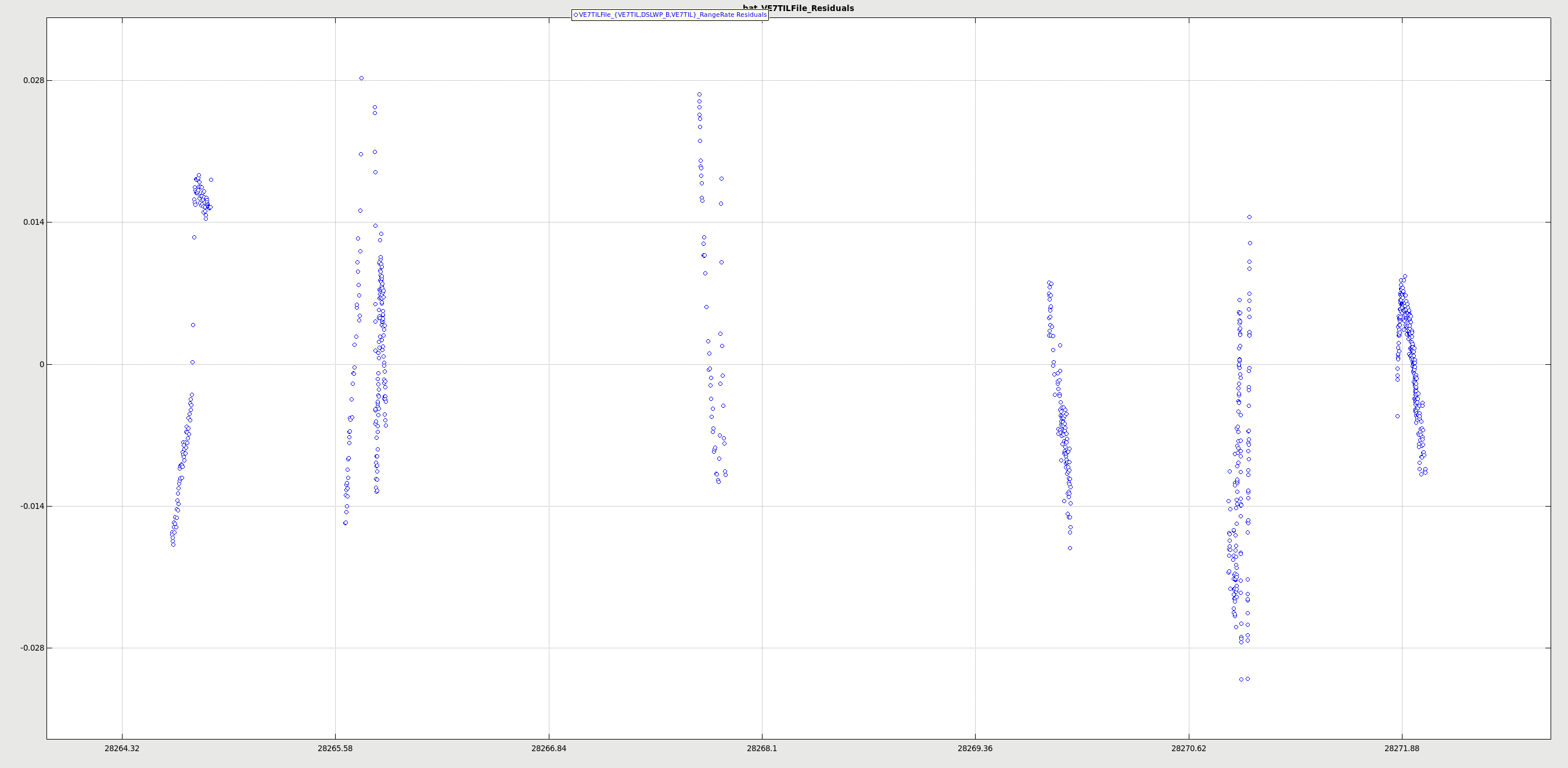
The normalized RMS error is about 3.5. This is higher than the desired value of 1, so it indicates that the orbit doesn’t fit our data so well, taking into account the error model we have provided. We will have to look at ways to improve data collection or data processing to reduce the error.
GMAT also produces the following plot for the residuals. Note that a residual of 0.028km/s of RangeRate corresponds to around 100Hz of residual in Doppler.
Let us now compare the orbit elements coming from the tracking file with the orbit elements produced by Doppler determination. For convenience, we list both again.
% State from tracking file
DSLWP_B.SMA = 8765.409054517644;
DSLWP_B.ECC = 0.7618824709853163;
DSLWP_B.INC = 20.80912899224475;
DSLWP_B.RAAN = 307.3706391221838;
DSLWP_B.AOP = 118.7406568683716;
DSLWP_B.TA = 178.2429103785479;

% State from orbit determination
DSLWP_B.SMA = 8761.0758581
DSLWP_B.ECC = 0.768016853537
DSLWP_B.INC = 16.9728174682
DSLWP_B.RAAN = 295.670653562
DSLWP_B.AOP = 130.427472407
DSLWP_B.TA = 178.126596496
We see that there is good agreement in the true anomaly. This is not a surprise, because it is easy to spot the time of periapsis in the Doppler data. The semi-major axis is 4.4km lower in the Doppler determination, implying a slightly faster orbit period. This is interesting because the 20180603 tracking file also shows a semi-major axis which is slightly lower than the other tracking files. I wonder if now that there are several days of measurements available, the DSLWP team at Harbin have used the measurements to refine the orbit period and this has shown up as a change in the 20180603 tracking file.
Other than that, the inclination, right-ascension of ascending element and argument of perigee show differences of a few degrees between the tracking file and the orbit determination. These parameters do not produce drastic changes in the Doppler curve, so it is not so easy to estimate them precisely.
Another thing that I wonder is to which extent is this estimation sensible in the 3400Hz shift I’ve applied to the Doppler data, since this shift has been estimated by eyesight.
After running the Doppler simulation again with the orbital elements obtained from the orbit determination, we get the following plot.
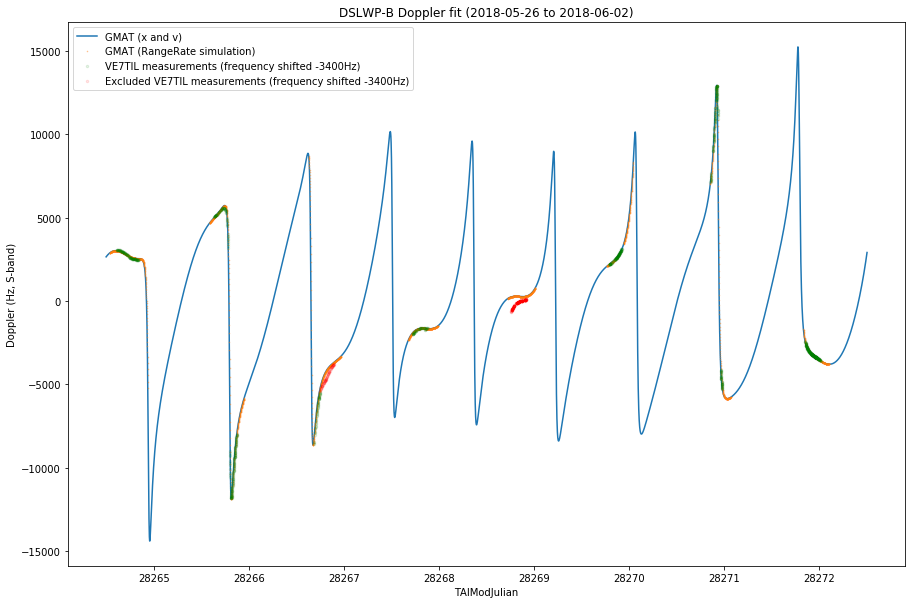
These calculations have been performed using this Jupyter notebook and this GMAT script.
It would be good to get more Doppler data from other stations and perhaps get the team at Harbin involved and share Doppler data and estimation techniques and results with them.
Interesantísimos artículos los que has publicado sobre esto. A veces me pierdo un poco (supongo que al usar el traductor) lo que demuestra el gran nivel que posees.
Me gustaría hacerte dos preguntas, si no te importa:
1) ¿Crees que con una estación para sat normalita (1 yagui de 9 el y preamp de 20 dB) podre recibir algo? (Imagino que como mucho en JT9G)
2) Como el pc del cuarto de radio es viejuno (va con win xp) y solo me corre el GMAT R2014, podría con solo apuntar a la Luna acertar a recibir este sat…o en su defecto, que aconsejas.
Gracias
Hola Carlos,
En las grabaciones de PI9CAM he visto hasta 15dB Eb/N0, estimados por el receptor de gr-dslwp. Esto son 36dB de C/N0 (a 125bps). JT4G requiere unos 16dB de C/N0 para ser decodificado, por tanto, se podría llegar a usar una estación unos 20dB peor que PI9CAM para el JT4G. El disco de 25m de PI9CAM tendrá unos 36dBi de ganancia en 436MHz (asumiendo un 50% de eficiencia). Por tanto necesitas alrededor de 16dBi de ganancia para JT4G. Esto es un yagi de unos 3m de boom, así que con 9 elementos lo veo bien difícil.
Para apuntar te basta con apuntar a la luna, ya que, visto desde la tierra, DSLWP-B no se aleja más de 2 o 3º de la luna. Lo que sí necesitas es realizar la corrección de Doppler (salvo que quieras andar buscando la señal en un rango de unos 6kHz), para lo cual te recomiendo que emplees los archivos de tracking publicados por Wei.